Code and Data Slides Template

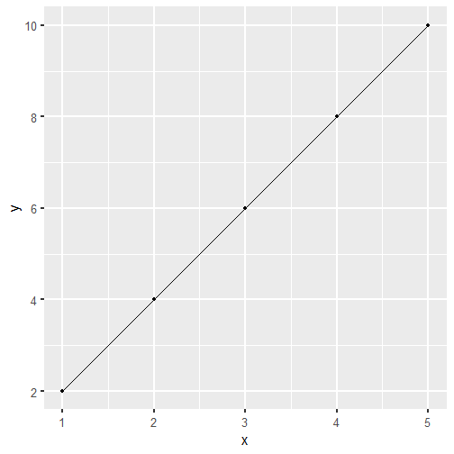
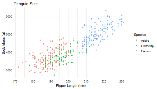
class: center, middle, inverse, title-slide

.title[
# Code and Data Slides Template
]
.author[
### S. Mason Garrison
]

---

# Simple Code Chunk

Here's a simple R code chunk:

``` r
x <- 3 * 4
y <- 10 - 2
z <- x + y
print(z)
```

```
## [1] 20
```

---

# Code with Output

This code chunk will show both the code and its output:

``` r
# Create a vector
numbers <- c(1, 2, 3, 4, 5)

# Calculate mean and standard deviation
mean_value <- mean(numbers)
sd_value <- sd(numbers)

# Print results
cat("Mean:", mean_value, "\n")
```

```
## Mean: 3
```

``` r
cat("Standard Deviation:", sd_value)
```

```
## Standard Deviation: 1.581139
```

---

# Code with Highlighted Lines

In this example, we'll highlight important lines:

``` r
# Load the tidyverse package
library(tidyverse)

# Create a simple dataframe
df <- tibble(
  x = 1:5,
  y = c(2, 4, 6, 8, 10)
)

# Plot the data
ggplot(df, aes(x, y)) +
  geom_point() +
  geom_line()
```

![](d00_code_files/figure-html/highlight-lines-1.png)

---

# Data Visualization Code

Here's an example of creating a data visualization with code:

``` r
conflicts_prefer(palmerpenguins::penguins,.quiet = TRUE)
ggplot(penguins, aes(x = flipper_length_mm, y = body_mass_g, color = species)) +
  geom_point(alpha = 0.7,na.rm=TRUE ) +
  labs(title = "Penguin Size",
       x = "Flipper Length (mm)",
       y = "Body Mass (g)",
       color = "Species") +
  theme_minimal()
```

![](d00_code_files/figure-html/data-viz-1.png)

---

# Data Manipulation

This slide demonstrates data manipulation with dplyr:

``` r
penguins %>%
  group_by(species, island) %>%
  summarize(
    mean_body_mass = mean(body_mass_g, na.rm = TRUE),
    mean_flipper_length = mean(flipper_length_mm, na.rm = TRUE)
  ) %>%
  arrange(desc(mean_body_mass))
```

```
## # A tibble: 5 × 4
## # Groups:   species [3]
##   species   island    mean_body_mass mean_flipper_length
##   <fct>     <fct>              <dbl>               <dbl>
## 1 Gentoo    Biscoe             5076.                217.
## 2 Chinstrap Dream              3733.                196.
## 3 Adelie    Biscoe             3710.                189.
## 4 Adelie    Torgersen          3706.                191.
## 5 Adelie    Dream              3688.                190.
```

---

# Interactive Code Output

This slide shows how to create an interactive table:

``` r
library(DT)

penguins %>%
  select(species, island, body_mass_g, flipper_length_mm) %>%
  datatable()
```

<div class="datatables html-widget html-fill-item" id="htmlwidget-c2e3fede5c798441fdae" style="width:100%;height:auto;"></div>
<script type="application/json" data-for="htmlwidget-c2e3fede5c798441fdae">{"x":{"filter":"none","vertical":false,"data":[["1","2","3","4","5","6","7","8","9","10","11","12","13","14","15","16","17","18","19","20","21","22","23","24","25","26","27","28","29","30","31","32","33","34","35","36","37","38","39","40","41","42","43","44","45","46","47","48","49","50","51","52","53","54","55","56","57","58","59","60","61","62","63","64","65","66","67","68","69","70","71","72","73","74","75","76","77","78","79","80","81","82","83","84","85","86","87","88","89","90","91","92","93","94","95","96","97","98","99","100","101","102","103","104","105","106","107","108","109","110","111","112","113","114","115","116","117","118","119","120","121","122","123","124","125","126","127","128","129","130","131","132","133","134","135","136","137","138","139","140","141","142","143","144","145","146","147","148","149","150","151","152","153","154","155","156","157","158","159","160","161","162","163","164","165","166","167","168","169","170","171","172","173","174","175","176","177","178","179","180","181","182","183","184","185","186","187","188","189","190","191","192","193","194","195","196","197","198","199","200","201","202","203","204","205","206","207","208","209","210","211","212","213","214","215","216","217","218","219","220","221","222","223","224","225","226","227","228","229","230","231","232","233","234","235","236","237","238","239","240","241","242","243","244","245","246","247","248","249","250","251","252","253","254","255","256","257","258","259","260","261","262","263","264","265","266","267","268","269","270","271","272","273","274","275","276","277","278","279","280","281","282","283","284","285","286","287","288","289","290","291","292","293","294","295","296","297","298","299","300","301","302","303","304","305","306","307","308","309","310","311","312","313","314","315","316","317","318","319","320","321","322","323","324","325","326","327","328","329","330","331","332","333","334","335","336","337","338","339","340","341","342","343","344"],["Adelie","Adelie","Adelie","Adelie","Adelie","Adelie","Adelie","Adelie","Adelie","Adelie","Adelie","Adelie","Adelie","Adelie","Adelie","Adelie","Adelie","Adelie","Adelie","Adelie","Adelie","Adelie","Adelie","Adelie","Adelie","Adelie","Adelie","Adelie","Adelie","Adelie","Adelie","Adelie","Adelie","Adelie","Adelie","Adelie","Adelie","Adelie","Adelie","Adelie","Adelie","Adelie","Adelie","Adelie","Adelie","Adelie","Adelie","Adelie","Adelie","Adelie","Adelie","Adelie","Adelie","Adelie","Adelie","Adelie","Adelie","Adelie","Adelie","Adelie","Adelie","Adelie","Adelie","Adelie","Adelie","Adelie","Adelie","Adelie","Adelie","Adelie","Adelie","Adelie","Adelie","Adelie","Adelie","Adelie","Adelie","Adelie","Adelie","Adelie","Adelie","Adelie","Adelie","Adelie","Adelie","Adelie","Adelie","Adelie","Adelie","Adelie","Adelie","Adelie","Adelie","Adelie","Adelie","Adelie","Adelie","Adelie","Adelie","Adelie","Adelie","Adelie","Adelie","Adelie","Adelie","Adelie","Adelie","Adelie","Adelie","Adelie","Adelie","Adelie","Adelie","Adelie","Adelie","Adelie","Adelie","Adelie","Adelie","Adelie","Adelie","Adelie","Adelie","Adelie","Adelie","Adelie","Adelie","Adelie","Adelie","Adelie","Adelie","Adelie","Adelie","Adelie","Adelie","Adelie","Adelie","Adelie","Adelie","Adelie","Adelie","Adelie","Adelie","Adelie","Adelie","Adelie","Adelie","Adelie","Adelie","Adelie","Adelie","Adelie","Gentoo","Gentoo","Gentoo","Gentoo","Gentoo","Gentoo","Gentoo","Gentoo","Gentoo","Gentoo","Gentoo","Gentoo","Gentoo","Gentoo","Gentoo","Gentoo","Gentoo","Gentoo","Gentoo","Gentoo","Gentoo","Gentoo","Gentoo","Gentoo","Gentoo","Gentoo","Gentoo","Gentoo","Gentoo","Gentoo","Gentoo","Gentoo","Gentoo","Gentoo","Gentoo","Gentoo","Gentoo","Gentoo","Gentoo","Gentoo","Gentoo","Gentoo","Gentoo","Gentoo","Gentoo","Gentoo","Gentoo","Gentoo","Gentoo","Gentoo","Gentoo","Gentoo","Gentoo","Gentoo","Gentoo","Gentoo","Gentoo","Gentoo","Gentoo","Gentoo","Gentoo","Gentoo","Gentoo","Gentoo","Gentoo","Gentoo","Gentoo","Gentoo","Gentoo","Gentoo","Gentoo","Gentoo","Gentoo","Gentoo","Gentoo","Gentoo","Gentoo","Gentoo","Gentoo","Gentoo","Gentoo","Gentoo","Gentoo","Gentoo","Gentoo","Gentoo","Gentoo","Gentoo","Gentoo","Gentoo","Gentoo","Gentoo","Gentoo","Gentoo","Gentoo","Gentoo","Gentoo","Gentoo","Gentoo","Gentoo","Gentoo","Gentoo","Gentoo","Gentoo","Gentoo","Gentoo","Gentoo","Gentoo","Gentoo","Gentoo","Gentoo","Gentoo","Gentoo","Gentoo","Gentoo","Gentoo","Gentoo","Gentoo","Gentoo","Gentoo","Gentoo","Gentoo","Gentoo","Gentoo","Chinstrap","Chinstrap","Chinstrap","Chinstrap","Chinstrap","Chinstrap","Chinstrap","Chinstrap","Chinstrap","Chinstrap","Chinstrap","Chinstrap","Chinstrap","Chinstrap","Chinstrap","Chinstrap","Chinstrap","Chinstrap","Chinstrap","Chinstrap","Chinstrap","Chinstrap","Chinstrap","Chinstrap","Chinstrap","Chinstrap","Chinstrap","Chinstrap","Chinstrap","Chinstrap","Chinstrap","Chinstrap","Chinstrap","Chinstrap","Chinstrap","Chinstrap","Chinstrap","Chinstrap","Chinstrap","Chinstrap","Chinstrap","Chinstrap","Chinstrap","Chinstrap","Chinstrap","Chinstrap","Chinstrap","Chinstrap","Chinstrap","Chinstrap","Chinstrap","Chinstrap","Chinstrap","Chinstrap","Chinstrap","Chinstrap","Chinstrap","Chinstrap","Chinstrap","Chinstrap","Chinstrap","Chinstrap","Chinstrap","Chinstrap","Chinstrap","Chinstrap","Chinstrap","Chinstrap"],["Torgersen","Torgersen","Torgersen","Torgersen","Torgersen","Torgersen","Torgersen","Torgersen","Torgersen","Torgersen","Torgersen","Torgersen","Torgersen","Torgersen","Torgersen","Torgersen","Torgersen","Torgersen","Torgersen","Torgersen","Biscoe","Biscoe","Biscoe","Biscoe","Biscoe","Biscoe","Biscoe","Biscoe","Biscoe","Biscoe","Dream","Dream","Dream","Dream","Dream","Dream","Dream","Dream","Dream","Dream","Dream","Dream","Dream","Dream","Dream","Dream","Dream","Dream","Dream","Dream","Biscoe","Biscoe","Biscoe","Biscoe","Biscoe","Biscoe","Biscoe","Biscoe","Biscoe","Biscoe","Biscoe","Biscoe","Biscoe","Biscoe","Biscoe","Biscoe","Biscoe","Biscoe","Torgersen","Torgersen","Torgersen","Torgersen","Torgersen","Torgersen","Torgersen","Torgersen","Torgersen","Torgersen","Torgersen","Torgersen","Torgersen","Torgersen","Torgersen","Torgersen","Dream","Dream","Dream","Dream","Dream","Dream","Dream","Dream","Dream","Dream","Dream","Dream","Dream","Dream","Dream","Dream","Biscoe","Biscoe","Biscoe","Biscoe","Biscoe","Biscoe","Biscoe","Biscoe","Biscoe","Biscoe","Biscoe","Biscoe","Biscoe","Biscoe","Biscoe","Biscoe","Torgersen","Torgersen","Torgersen","Torgersen","Torgersen","Torgersen","Torgersen","Torgersen","Torgersen","Torgersen","Torgersen","Torgersen","Torgersen","Torgersen","Torgersen","Torgersen","Dream","Dream","Dream","Dream","Dream","Dream","Dream","Dream","Dream","Dream","Dream","Dream","Dream","Dream","Dream","Dream","Dream","Dream","Dream","Dream","Biscoe","Biscoe","Biscoe","Biscoe","Biscoe","Biscoe","Biscoe","Biscoe","Biscoe","Biscoe","Biscoe","Biscoe","Biscoe","Biscoe","Biscoe","Biscoe","Biscoe","Biscoe","Biscoe","Biscoe","Biscoe","Biscoe","Biscoe","Biscoe","Biscoe","Biscoe","Biscoe","Biscoe","Biscoe","Biscoe","Biscoe","Biscoe","Biscoe","Biscoe","Biscoe","Biscoe","Biscoe","Biscoe","Biscoe","Biscoe","Biscoe","Biscoe","Biscoe","Biscoe","Biscoe","Biscoe","Biscoe","Biscoe","Biscoe","Biscoe","Biscoe","Biscoe","Biscoe","Biscoe","Biscoe","Biscoe","Biscoe","Biscoe","Biscoe","Biscoe","Biscoe","Biscoe","Biscoe","Biscoe","Biscoe","Biscoe","Biscoe","Biscoe","Biscoe","Biscoe","Biscoe","Biscoe","Biscoe","Biscoe","Biscoe","Biscoe","Biscoe","Biscoe","Biscoe","Biscoe","Biscoe","Biscoe","Biscoe","Biscoe","Biscoe","Biscoe","Biscoe","Biscoe","Biscoe","Biscoe","Biscoe","Biscoe","Biscoe","Biscoe","Biscoe","Biscoe","Biscoe","Biscoe","Biscoe","Biscoe","Biscoe","Biscoe","Biscoe","Biscoe","Biscoe","Biscoe","Biscoe","Biscoe","Biscoe","Biscoe","Biscoe","Biscoe","Biscoe","Biscoe","Biscoe","Biscoe","Biscoe","Biscoe","Biscoe","Biscoe","Biscoe","Biscoe","Biscoe","Biscoe","Dream","Dream","Dream","Dream","Dream","Dream","Dream","Dream","Dream","Dream","Dream","Dream","Dream","Dream","Dream","Dream","Dream","Dream","Dream","Dream","Dream","Dream","Dream","Dream","Dream","Dream","Dream","Dream","Dream","Dream","Dream","Dream","Dream","Dream","Dream","Dream","Dream","Dream","Dream","Dream","Dream","Dream","Dream","Dream","Dream","Dream","Dream","Dream","Dream","Dream","Dream","Dream","Dream","Dream","Dream","Dream","Dream","Dream","Dream","Dream","Dream","Dream","Dream","Dream","Dream","Dream","Dream","Dream"],[3750,3800,3250,null,3450,3650,3625,4675,3475,4250,3300,3700,3200,3800,4400,3700,3450,4500,3325,4200,3400,3600,3800,3950,3800,3800,3550,3200,3150,3950,3250,3900,3300,3900,3325,4150,3950,3550,3300,4650,3150,3900,3100,4400,3000,4600,3425,2975,3450,4150,3500,4300,3450,4050,2900,3700,3550,3800,2850,3750,3150,4400,3600,4050,2850,3950,3350,4100,3050,4450,3600,3900,3550,4150,3700,4250,3700,3900,3550,4000,3200,4700,3800,4200,3350,3550,3800,3500,3950,3600,3550,4300,3400,4450,3300,4300,3700,4350,2900,4100,3725,4725,3075,4250,2925,3550,3750,3900,3175,4775,3825,4600,3200,4275,3900,4075,2900,3775,3350,3325,3150,3500,3450,3875,3050,4000,3275,4300,3050,4000,3325,3500,3500,4475,3425,3900,3175,3975,3400,4250,3400,3475,3050,3725,3000,3650,4250,3475,3450,3750,3700,4000,4500,5700,4450,5700,5400,4550,4800,5200,4400,5150,4650,5550,4650,5850,4200,5850,4150,6300,4800,5350,5700,5000,4400,5050,5000,5100,4100,5650,4600,5550,5250,4700,5050,6050,5150,5400,4950,5250,4350,5350,3950,5700,4300,4750,5550,4900,4200,5400,5100,5300,4850,5300,4400,5000,4900,5050,4300,5000,4450,5550,4200,5300,4400,5650,4700,5700,4650,5800,4700,5550,4750,5000,5100,5200,4700,5800,4600,6000,4750,5950,4625,5450,4725,5350,4750,5600,4600,5300,4875,5550,4950,5400,4750,5650,4850,5200,4925,4875,4625,5250,4850,5600,4975,5500,4725,5500,4700,5500,4575,5500,5000,5950,4650,5500,4375,5850,4875,6000,4925,null,4850,5750,5200,5400,3500,3900,3650,3525,3725,3950,3250,3750,4150,3700,3800,3775,3700,4050,3575,4050,3300,3700,3450,4400,3600,3400,2900,3800,3300,4150,3400,3800,3700,4550,3200,4300,3350,4100,3600,3900,3850,4800,2700,4500,3950,3650,3550,3500,3675,4450,3400,4300,3250,3675,3325,3950,3600,4050,3350,3450,3250,4050,3800,3525,3950,3650,3650,4000,3400,3775,4100,3775],[181,186,195,null,193,190,181,195,193,190,186,180,182,191,198,185,195,197,184,194,174,180,189,185,180,187,183,187,172,180,178,178,188,184,195,196,190,180,181,184,182,195,186,196,185,190,182,179,190,191,186,188,190,200,187,191,186,193,181,194,185,195,185,192,184,192,195,188,190,198,190,190,196,197,190,195,191,184,187,195,189,196,187,193,191,194,190,189,189,190,202,205,185,186,187,208,190,196,178,192,192,203,183,190,193,184,199,190,181,197,198,191,193,197,191,196,188,199,189,189,187,198,176,202,186,199,191,195,191,210,190,197,193,199,187,190,191,200,185,193,193,187,188,190,192,185,190,184,195,193,187,201,211,230,210,218,215,210,211,219,209,215,214,216,214,213,210,217,210,221,209,222,218,215,213,215,215,215,216,215,210,220,222,209,207,230,220,220,213,219,208,208,208,225,210,216,222,217,210,225,213,215,210,220,210,225,217,220,208,220,208,224,208,221,214,231,219,230,214,229,220,223,216,221,221,217,216,230,209,220,215,223,212,221,212,224,212,228,218,218,212,230,218,228,212,224,214,226,216,222,203,225,219,228,215,228,216,215,210,219,208,209,216,229,213,230,217,230,217,222,214,null,215,222,212,213,192,196,193,188,197,198,178,197,195,198,193,194,185,201,190,201,197,181,190,195,181,191,187,193,195,197,200,200,191,205,187,201,187,203,195,199,195,210,192,205,210,187,196,196,196,201,190,212,187,198,199,201,193,203,187,197,191,203,202,194,206,189,195,207,202,193,210,198]],"container":"<table class=\"display\">\n  <thead>\n    <tr>\n      <th> <\/th>\n      <th>species<\/th>\n      <th>island<\/th>\n      <th>body_mass_g<\/th>\n      <th>flipper_length_mm<\/th>\n    <\/tr>\n  <\/thead>\n<\/table>","options":{"columnDefs":[{"className":"dt-right","targets":[3,4]},{"orderable":false,"targets":0},{"name":" ","targets":0},{"name":"species","targets":1},{"name":"island","targets":2},{"name":"body_mass_g","targets":3},{"name":"flipper_length_mm","targets":4}],"order":[],"autoWidth":false,"orderClasses":false},"selection":{"mode":"multiple","selected":null,"target":"row","selectable":null}},"evals":[],"jsHooks":[]}</script>

---

# Code and Plot Side by Side

.pull-left[

``` r
ggplot(mtcars, aes(x = wt, y = mpg)) +
  geom_point() +
  geom_smooth(method = "lm", se = FALSE,formula='y~x') +
  labs(
    title = "Car Weight vs. Miles Per Gallon",
    x = "Weight (1000 lbs)",
    y = "Miles Per Gallon"
  )
```
]

.pull-right[
<img src="d00_code_files/figure-html/unnamed-chunk-1-1.png" width="100%" />
]

---

# Statistical Analysis

This slide demonstrates a simple statistical test:

``` r
# Perform a t-test
t_test_result <- t.test(flipper_length_mm ~  sex, data = penguins)

# Print the results
print(t_test_result)
```

```
## 
## 	Welch Two Sample t-test
## 
## data:  flipper_length_mm by sex
## t = -4.8079, df = 325.28, p-value = 2.336e-06
## alternative hypothesis: true difference in means between group female and group male is not equal to 0
## 95 percent confidence interval:
##  -10.064811  -4.219821
## sample estimates:
## mean in group female   mean in group male 
##             197.3636             204.5060
```

---

## Residuals Plot

.pull-left[

``` r
depth_length_fit <- linear_reg() %>%
  set_engine("lm") %>%
  fit(bill_depth_mm ~ bill_length_mm, data = penguins)

depth_length_fit_aug <- augment(depth_length_fit$fit)

ggplot(depth_length_fit_aug, mapping = aes(x = .fitted, y = .resid)) +
  geom_point(alpha = 0.5) +
  geom_hline(yintercept = 0, color = "#bf2986ff", lty = "dashed") +
  labs(x = "Predicted Height", y = "Residuals")
```
]
.pull-right[
<img src="d00_code_files/figure-html/unnamed-chunk-2-1.png" width="100%" />
]

---

## Model Output

``` r
linear_reg() %>%
  set_engine("lm") %>%
  fit(bill_depth_mm ~ bill_length_mm, data = penguins) %>%
  tidy()
```

```
## # A tibble: 2 × 5
##   term           estimate std.error statistic  p.value
##   <chr>             <dbl>     <dbl>     <dbl>    <dbl>
## 1 (Intercept)     20.9       0.844      24.7  4.72e-78
## 2 bill_length_mm  -0.0850    0.0191     -4.46 1.12e- 5
```

---

## Data Exploration

.pull-left[

``` r
ggplot(penguins, aes(x = bill_depth_mm)) +
  geom_histogram(binwidth = 5) +
  labs(x = "Bill Depth (mm)", y = NULL)
```

```
## Warning: Removed 2 rows containing non-finite outside the scale range
## (`stat_bin()`).
```
]
.pull-right[

```
## Warning: Removed 2 rows containing non-finite outside the scale range
## (`stat_bin()`).
```

<img src="d00_code_files/figure-html/unnamed-chunk-3-1.png" width="100%" />
]