The projects should be numbered consecutively (i.e., in the order in which you began them), and should include for each project a description of the goal, the product (computer program, hand graph, computer graph, etc.), the data, and some interpretation. Reports must be reproducible and of high quality in terms of writing, grammar, presentation, etc.

This template shows how to source code from an R script, and how to include the output in the report. The code is in p02/scripts/script.R, and the output is included below.

Overview

This example demonstrates how to use source() to load reusable R functions from a separate script.

In this template, the sourced script is located here:

script_path <- "p02/scripts/scripts.R"

script_path

## [1] "p02/scripts/scripts.R"

The script contains functions for:

applying a consistent plot theme
adding plot labels
summarizing numeric variables
making histograms
making scatterplots
fitting a simple regression model
summarizing model results

Source the Functions

The function source() runs the R script and loads the functions from that script into the current R session.

source(script_path)

After this code runs, the functions from theme_functions.R are available in this R Markdown document.

Load Example Data

This example uses the built-in mtcars dataset as well as data in the data folder of the template. The data() function loads the mtcars dataset. The read.csv() function loads the data from the CSV file.

data(mtcars)

head(mtcars)

##                    mpg cyl disp  hp drat    wt  qsec vs am gear carb
## Mazda RX4         21.0   6  160 110 3.90 2.620 16.46  0  1    4    4
## Mazda RX4 Wag     21.0   6  160 110 3.90 2.875 17.02  0  1    4    4
## Datsun 710        22.8   4  108  93 3.85 2.320 18.61  1  1    4    1
## Hornet 4 Drive    21.4   6  258 110 3.08 3.215 19.44  1  0    3    1
## Hornet Sportabout 18.7   8  360 175 3.15 3.440 17.02  0  0    3    2
## Valiant           18.1   6  225 105 2.76 3.460 20.22  1  0    3    1

portfolio_data <- read.csv("p02/data/portfolio_example_data.csv")

Cars examples

Summarize a Numeric Variable

The function summarize_numeric() comes from the sourced script.

summarize_numeric(
  data = mtcars,
  variable = "mpg"
)

##   variable     mean standard_deviation minimum median maximum
## 1      mpg 20.09062           6.026948    10.4   19.2    33.9

The same function can be reused for a different variable.

summarize_numeric(
  data = mtcars,
  variable = "wt"
)

##   variable    mean standard_deviation minimum median maximum
## 1       wt 3.21725          0.9784574   1.513  3.325   5.424

Or a different dataset.

summarize_numeric(portfolio_data, "temperature_f")

##        variable   mean standard_deviation minimum median maximum
## 1 temperature_f 66.864           12.64044    26.2  67.25   115.1

summarize_numeric(portfolio_data, "pm25")

##   variable   mean standard_deviation minimum median maximum
## 1     pm25 20.755           5.771449     6.5     21    36.2

Plots

Make a Histogram

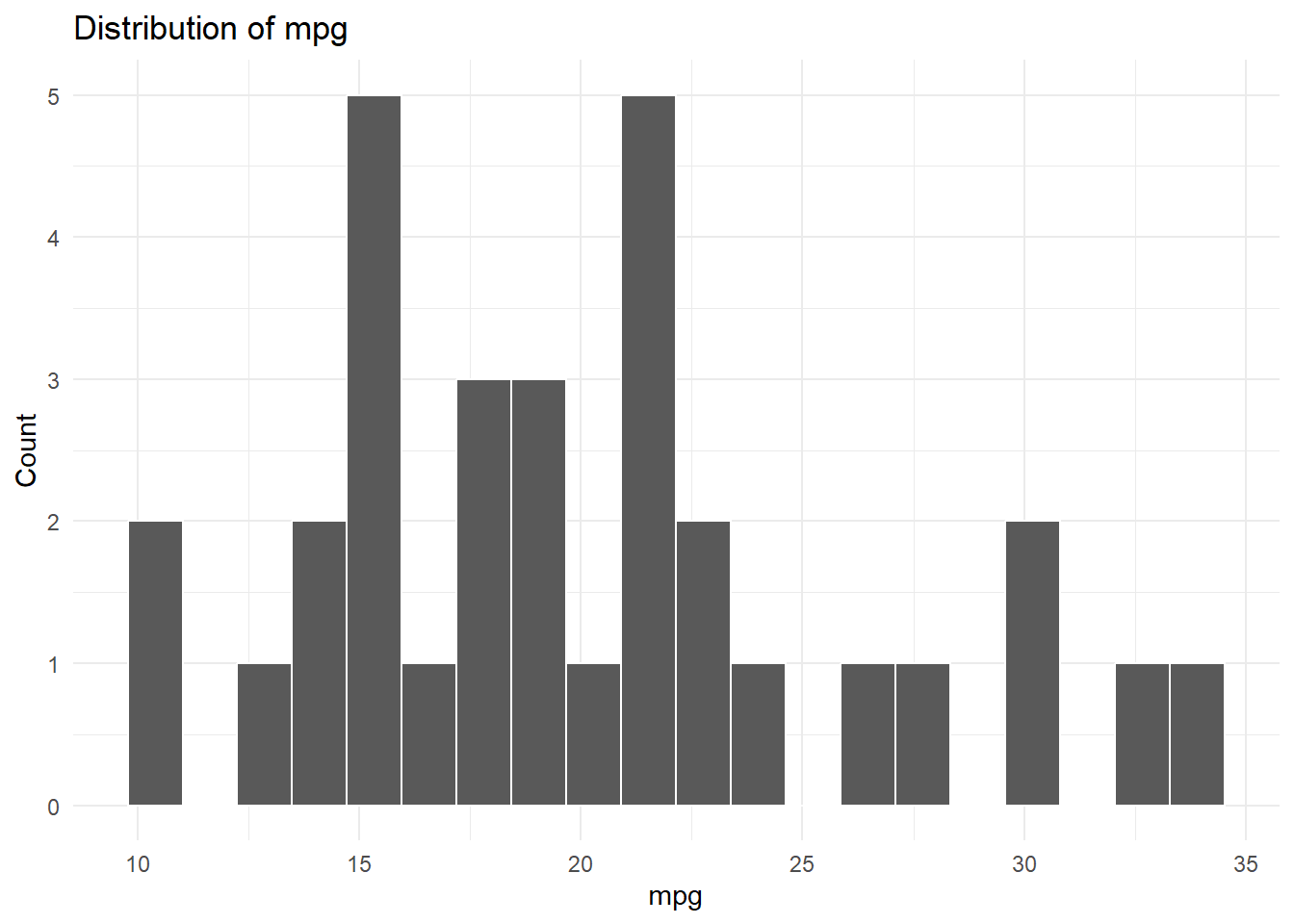
The function make_histogram() creates a histogram for a selected variable.

make_histogram(
  data = mtcars,
  variable = "mpg"
)

make_histogram(portfolio_data, "pm25")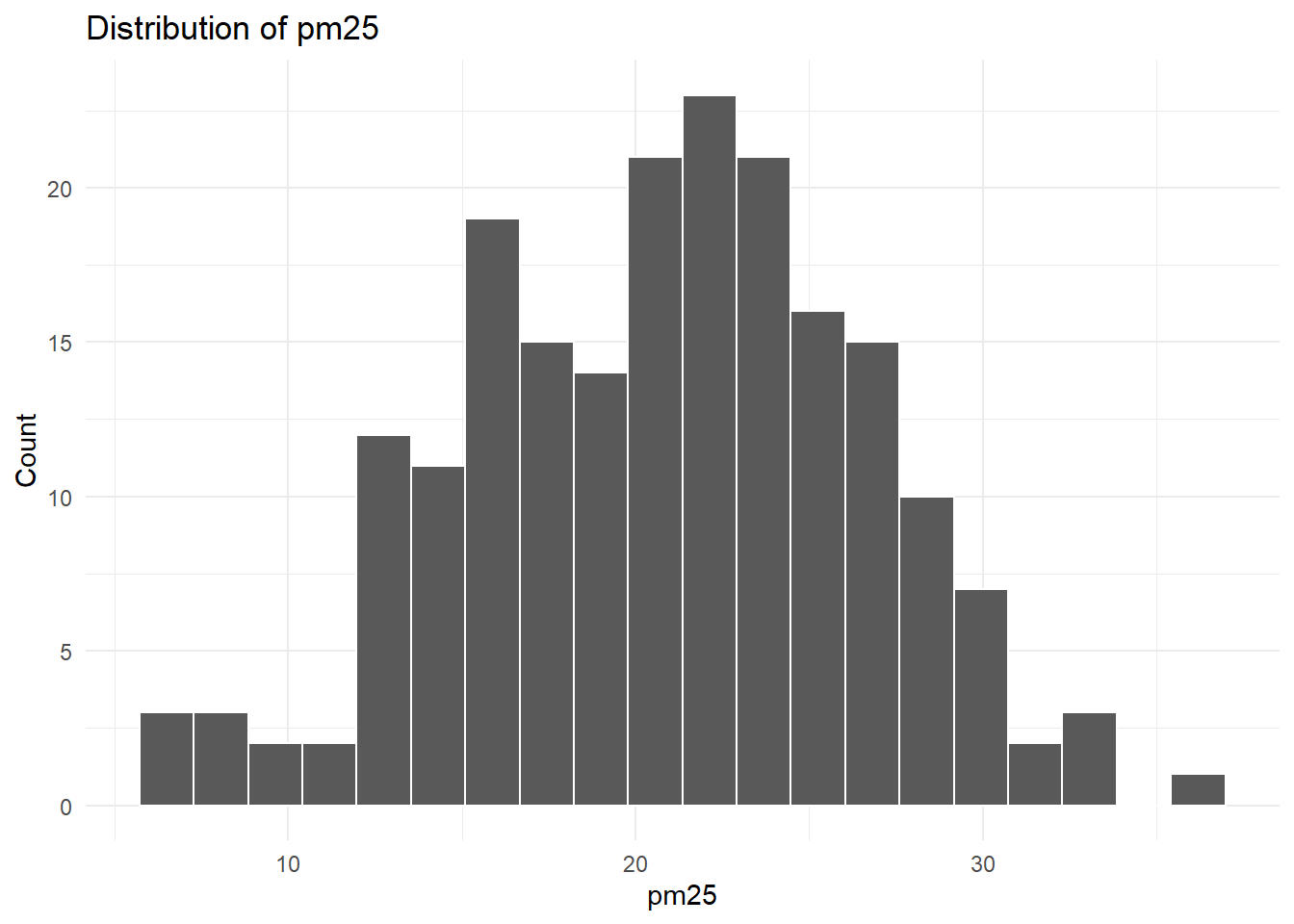

The plot can also be modified after the function creates it.

make_histogram(portfolio_data, "pm25") +
  theme_portfolio()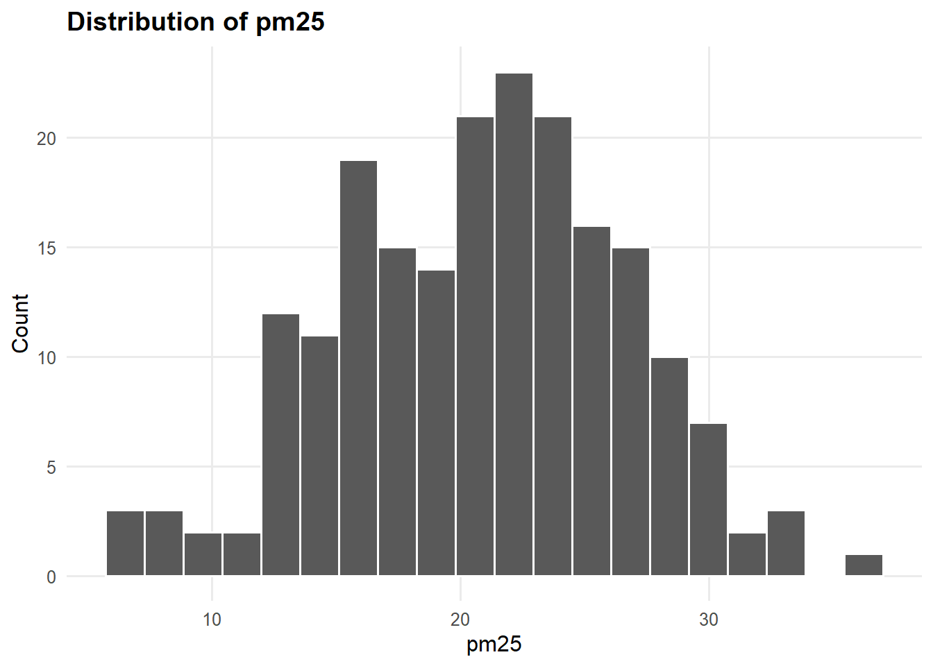

Make a Scatterplot

The function make_scatterplot() creates a scatterplot using two variables.

p1 <- make_scatterplot(
  data = mtcars,
  x_variable = "wt",
  y_variable = "mpg"
)

p1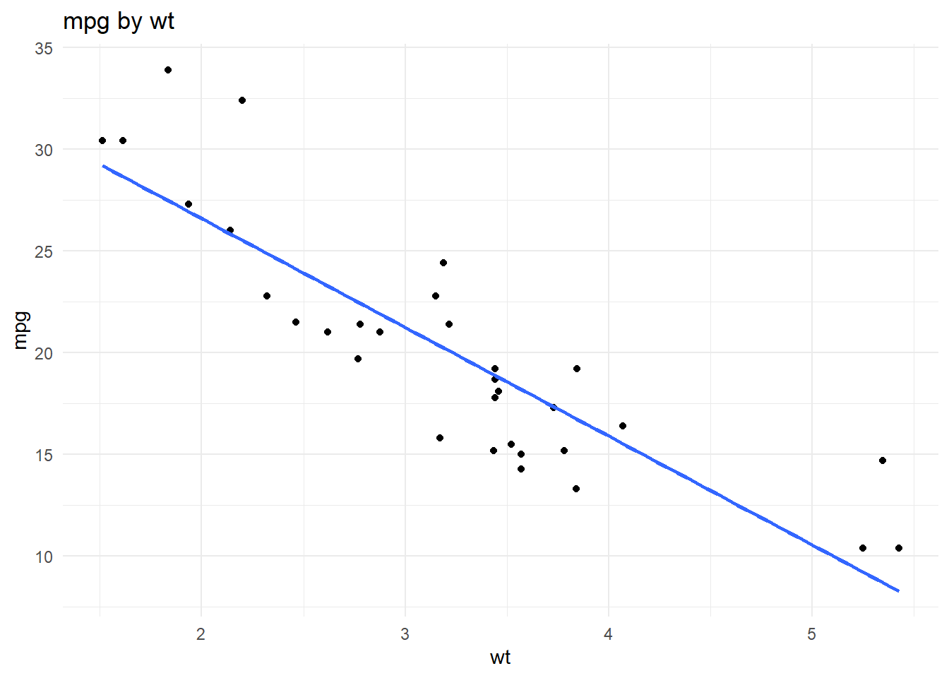

We can compare the scatterplot from the mtcars dataset to a scatterplot from the portfolio_data dataset, using Cowplot to arrange them side by side.

library(cowplot)
p2 <- make_scatterplot(
  data = portfolio_data,
  x_variable = "traffic_index",
  y_variable = "pm25"
)

cowplot::plot_grid(p1, p2, labels = c("A", "B"))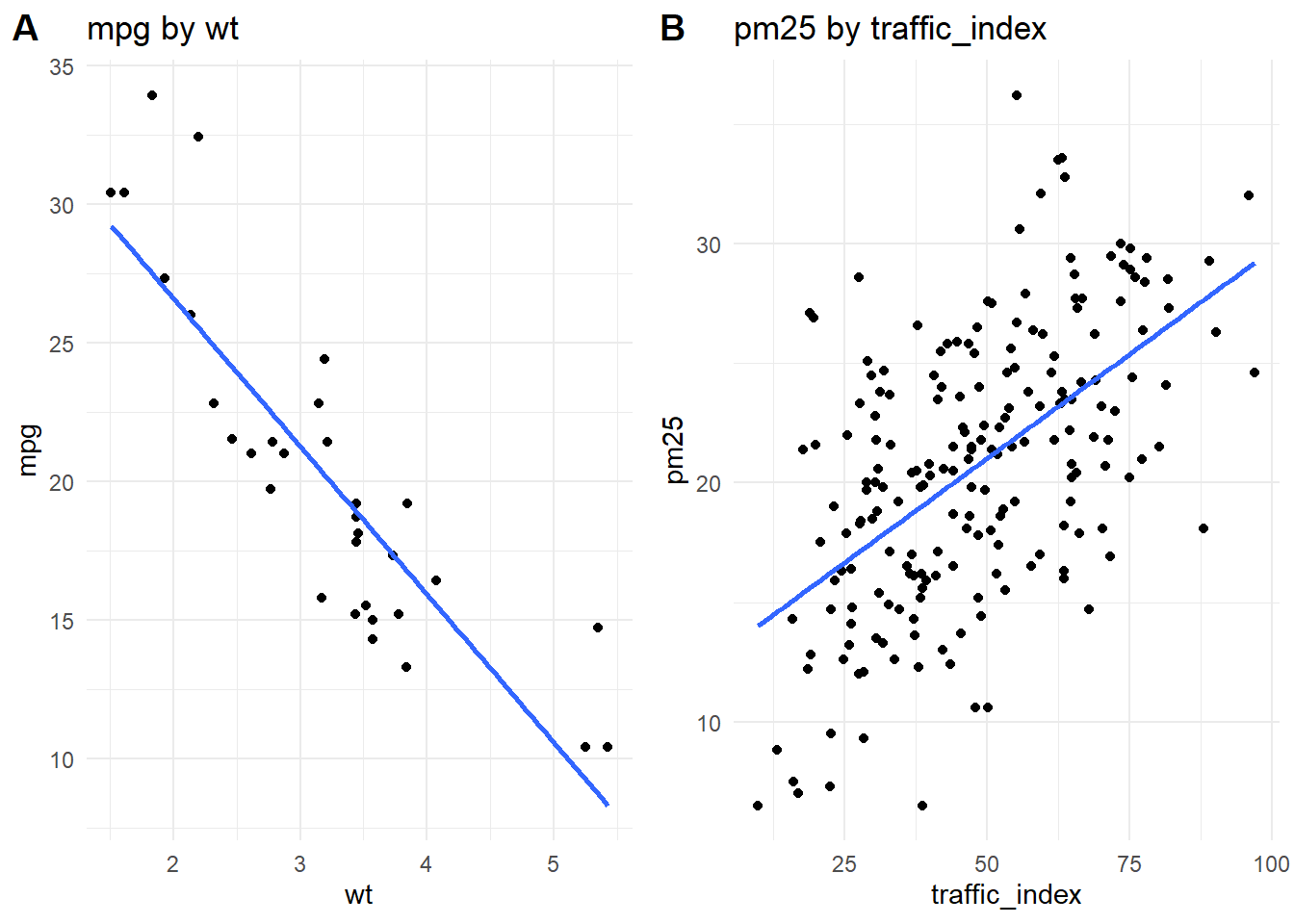

The sourced function gives us a basic plot. We can then add other sourced functions to modify it.

scatterplot <- make_scatterplot(
  data = mtcars,
  x_variable = "wt",
  y_variable = "mpg"
)

scatterplot <- add_portfolio_labels(
  plot = scatterplot,
  title = "Fuel Efficiency by Vehicle Weight",
  subtitle = "Example using the built-in mtcars dataset",
  x = "Vehicle weight",
  y = "Miles per gallon",
  caption = "Data source: mtcars dataset in base R."
)

scatterplot + theme_portfolio()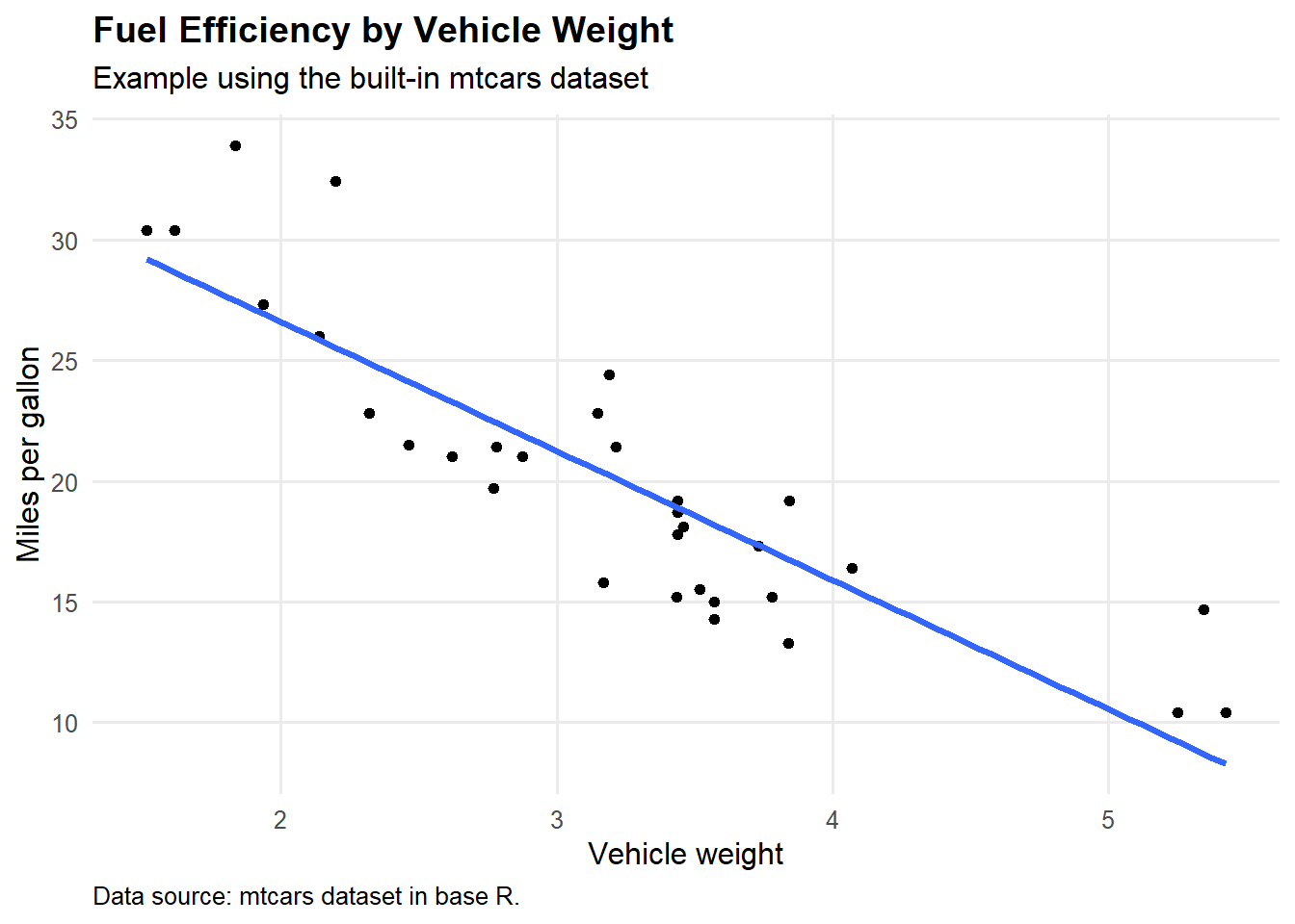

Fit a Simple Regression Model

The function fit_simple_regression() fits a linear regression model using variable names supplied as text.

mpg_model <- fit_simple_regression(
  data = mtcars,
  outcome = "mpg",
  predictor = "wt"
)

mpg_model

## 
## Call:
## lm(formula = model_formula, data = data)
## 
## Coefficients:
## (Intercept)           wt  
##      37.285       -5.344

Summarize the Model

The function summarize_model() extracts the coefficient table from the regression model.

summarize_model(mpg_model)

##          term  estimate standard_error test_statistic      p_value
## 1 (Intercept) 37.285126       1.877627      19.857575 8.241799e-19
## 2          wt -5.344472       0.559101      -9.559044 1.293959e-10

Use Model Results in Writing

The model can also be summarized directly in the text of the portfolio.

model_summary <- summarize_model(mpg_model)

slope <- model_summary$estimate[model_summary$term == "wt"]

In this model, the estimated slope for vehicle weight is -5.34. This means that, in the mtcars dataset, higher vehicle weight is associated with lower miles per gallon.

Why This Is Useful

Using source() allows us to keep reusable code in one script and use it throughout the portfolio.

For example, instead of rewriting the code for a histogram, a scatterplot, or a regression model in every section of the portfolio, we can write the function once in scripts/theme_functions.R and then call the function whenever we need it.

Template Structure

This example assumes the following folder structure:

portfolio-template/
  p02.Rmd
  p02/
    data/
      portfolio_example_data.csv
    scripts/
      scripts.R

Session Information

Including session information can help document the computational environment used to render the portfolio.

sessionInfo()

## R version 4.5.3 (2026-03-11 ucrt)
## Platform: x86_64-w64-mingw32/x64
## Running under: Windows 11 x64 (build 26200)
## 
## Matrix products: default
##   LAPACK version 3.12.1
## 
## locale:
## [1] LC_COLLATE=English_United States.utf8 
## [2] LC_CTYPE=English_United States.utf8   
## [3] LC_MONETARY=English_United States.utf8
## [4] LC_NUMERIC=C                          
## [5] LC_TIME=English_United States.utf8    
## 
## time zone: America/New_York
## tzcode source: internal
## 
## attached base packages:
## [1] stats     graphics  grDevices utils     datasets  methods   base     
## 
## other attached packages:
##  [1] cowplot_1.2.0   synthpop_1.9-2  lubridate_1.9.5 forcats_1.0.1  
##  [5] stringr_1.6.0   dplyr_1.2.1     purrr_1.2.2     readr_2.2.0    
##  [9] tidyr_1.3.2     tibble_3.3.1    ggplot2_4.0.2   tidyverse_2.0.0
## 
## loaded via a namespace (and not attached):
##  [1] tidyselect_1.2.1     libcoin_1.0-12       farver_2.1.2        
##  [4] S7_0.2.1-1           fastmap_1.2.0        TH.data_1.1-5       
##  [7] digest_0.6.39        rpart_4.1.27         timechange_0.4.0    
## [10] lifecycle_1.0.5      survival_3.8-6       Rsolnp_2.0.1        
## [13] magrittr_2.0.5       compiler_4.5.3       rlang_1.2.0         
## [16] sass_0.4.10          tools_4.5.3          yaml_2.3.12         
## [19] knitr_1.51           labeling_0.4.3       classInt_0.4-11     
## [22] plyr_1.8.9           RColorBrewer_1.1-3   multcomp_1.4-30     
## [25] KernSmooth_2.23-26   polspline_1.1.25     party_1.3-20        
## [28] numDeriv_2016.8-1.1  withr_3.0.2          foreign_0.8-91      
## [31] nnet_7.3-20          grid_4.5.3           mipfp_3.2.1         
## [34] stats4_4.5.3         broman_0.92          e1071_1.7-17        
## [37] future_1.70.0        globals_0.19.1       scales_1.4.0        
## [40] MASS_7.3-65          dichromat_2.0-0.1    cli_3.6.6           
## [43] mvtnorm_1.3-7        rmarkdown_2.31       generics_0.1.4      
## [46] otel_0.2.0           rstudioapi_0.18.0    future.apply_1.20.2 
## [49] tzdb_0.5.0           cachem_1.1.0         proxy_0.4-29        
## [52] modeltools_0.2-24    splines_4.5.3        parallel_4.5.3      
## [55] matrixStats_1.5.0    vctrs_0.7.3          Matrix_1.7-5        
## [58] sandwich_3.1-1       jsonlite_2.0.0       hms_1.1.4           
## [61] rmutil_1.1.10        cmm_1.0              listenv_0.10.1      
## [64] jquerylib_0.1.4      proto_1.0.0          glue_1.8.1          
## [67] parallelly_1.47.0    codetools_0.2-20     stringi_1.8.7       
## [70] strucchange_1.5-4    gtable_0.3.6         pillar_1.11.1       
## [73] htmltools_0.5.9      randomForest_4.7-1.2 truncnorm_1.0-9     
## [76] R6_2.6.1             evaluate_1.0.5       lattice_0.22-9      
## [79] bslib_0.10.0         class_7.3-23         Rcpp_1.1.1-1        
## [82] nlme_3.1-169         mgcv_1.9-4           ranger_0.18.0       
## [85] coin_1.4-3           xfun_0.57            zoo_1.8-15          
## [88] pkgconfig_2.0.3

Portfolio 2