48 Define mean and covariance matrix

mean_traits <- c(50, 50) cov_matrix_bigfive <- matrix(c(100, 50, 50, 100), ncol = 2)

Exercise 3: Preparing for the Unexpected

In space colonization, just like in any complex project management, it’s essential to prepare for variability and uncertainty. To test the resilience of our simulated Mars colony, we’ll generate multiple sets of potential colonists. By examining these various batches, we can assess how robust our colony’s attributes are and whether they can adapt to different scenarios.

48.0.1 Setting Up the Simulation

In this task, we will simulate interdependent skills using the mvrnorm function from the MASS package. This function allows us to generate data from a multivariate normal distribution, giving us control over the means, variances, and covariances of the simulated variables—ideal for modeling complex skill relationships among colonists.

library(MASS)  # Ensure the MASS package is loaded for mvrnorm

Parameters for Simulation

Define the mean skills levels and a covariance matrix to simulate technical skills and problem-solving abilities with a realistic correlation:

mean_skills <- c(50, 50)  # Mean technical skills and problem-solving abilities
cov_skills <- matrix(c(100, 50, 50, 100), ncol = 2)  # Covariance matrix showing how these skills correlate

48.0.2 Simulating Data

Generate the skills for 100 colonists, repeating this process multiple times to analyze the consistency and resilience of skill distribution:

set.seed(124)
num_simulations <- 100  # Number of times to simulate the colonist data
all_simulations <- replicate(num_simulations, mvrnorm(n = 100, mu = mean_skills, Sigma = cov_skills, empirical = TRUE))

set.seed(124)
sample_sizes <- seq(30, 300, by = 15)  # Varying sample sizes
repetitions_per_condition <- 20  # Number of repetitions for each sample size

# Initialize a DataFrame to store results
simulation_results <- data.frame(
  Condition = integer(),
  SampleSize = integer(),
  Repetition = integer(),
  Covariance = numeric()
)

# Nested loop for simulations
for (size in sample_sizes) {
  for (rep in 1:repetitions_per_condition) {
    skills_data <- mvrnorm(n = size, mu = mean_skills, Sigma = cov_skills, empirical = TRUE)
    current_covariance <- cov(skills_data[, 1], skills_data[, 2])
  
    # Append results
    simulation_results <- rbind(simulation_results, data.frame(
      SampleSize = size,
      Repetition = rep,
      Covariance = current_covariance
    ))
  }
}

library(ggplot2)

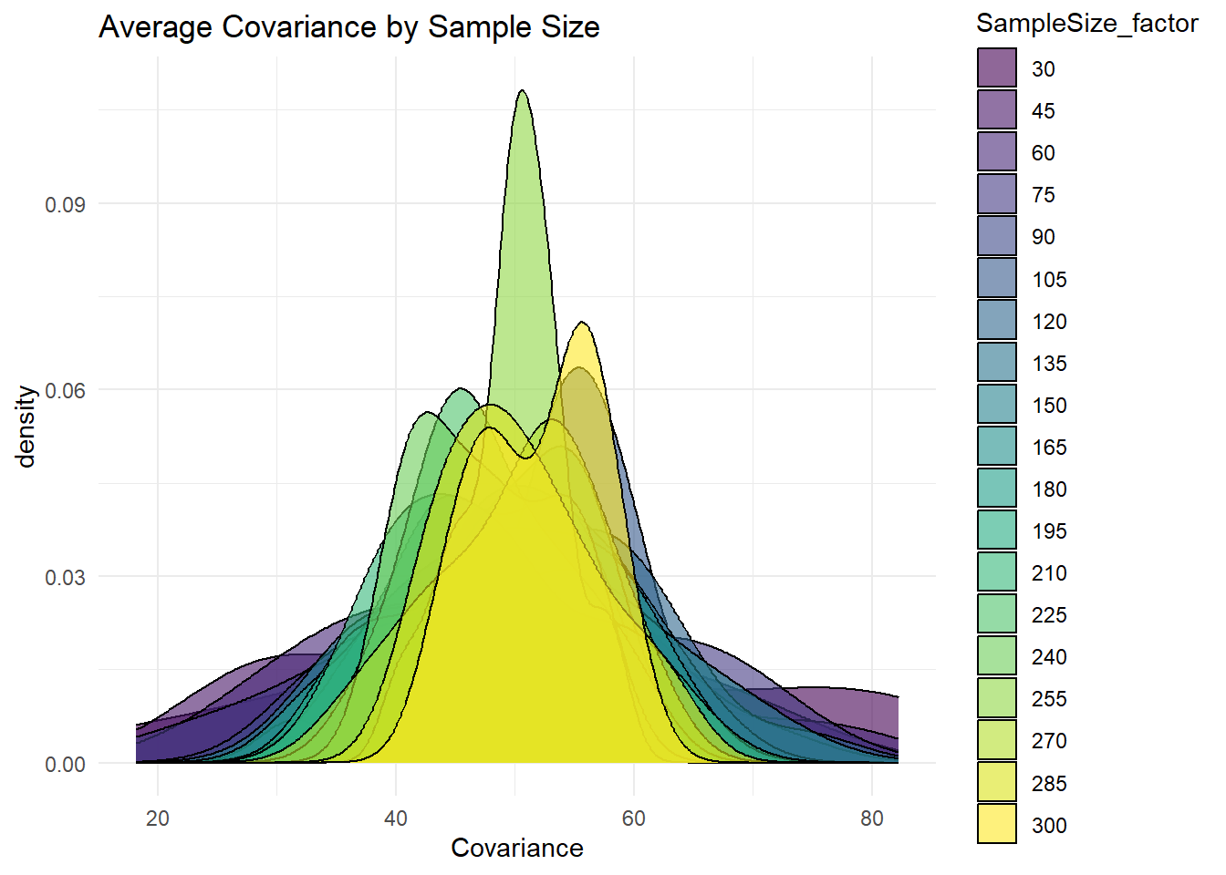
# Plotting the average covariance for each sample size
average_covariances <- simulation_results %>%
  group_by(SampleSize) %>%
  summarize(AverageCovariance = mean(Covariance))

ggplot(average_covariances, aes(x = SampleSize, y = AverageCovariance)) +
  geom_line() + 
  geom_point() +
  theme_minimal() +
  ggtitle("Average Covariance by Sample Size") +
  xlab("Sample Size") +
  ylab("Average Covariance")