87 LAB: Cross Validation in Action
Don’t Judge the Ship After It Sinks
In 1912, the RMS Titanic sank on its maiden voyage, killing over 1,500 of the roughly 2,200 people on board. The disaster sent shockwaves through the maritime insurance industry. Lloyd’s of London, the world’s oldest and most famous insurance market, had underwritten a significant portion of the Titanic’s hull and cargo. The claims that followed forced insurers to confront an uncomfortable question: could the risk have been quantified in advance?
We’ve been hired by Lloyd’s to help answer a version of that question retrospectively. Using passenger records, we will build classification models that predict survival and then evaluate how trustworthy those predictions really are. Along the way, you will discover a fundamental problem in predictive modeling: a model that looks good on data it has already seen may perform poorly on data it has not. Cross validation is a classic remedy, and this lab will teach you why it works and how to implement it.
Learning goals
- Fit and interpret logistic regression classifiers for binary outcomes in R.
- Compute predicted probabilities, convert them into class predictions, and calculate accuracy.
- Explain why apparent (in-sample) accuracy is optimistic.
- Evaluate models using held-out data and implement k-fold cross validation.
- Reason about how the choice of probability cutoff affects classification decisions.
- Handle missing data responsibly and avoid information leakage in evaluation pipelines.
Getting started and warming up
Go to the course GitHub organization and locate the lab repo, which should be named something like lab-11-cross-validation. Either Fork it or use the template. Then clone it in RStudio. First, open the R Markdown document lab-11.Rmd and Knit it. Make sure it compiles without errors.
The data
We will work with two Titanic datasets that complement each other:
titanic_trainandtitanic_testfrom thetitanicpackage (a convenient train/test split often used in Kaggle contexts). The training set includes 891 passengers with known survival outcomes; the test set has 418 passengers.titanic3loaded from data/titanic3.xls, which includes additional fields such asboat(lifeboat number),body(body identification number), andhome.dest(home/destination). This version contains 1,309 passengers total. Originally from here.
We will have to combine these datasets at some point, but for now we will keep them separate to illustrate the difference between training and test data.
titanic3 <- read_excel("data/titanic3.xls",
    col_types = c("numeric", "numeric", "text",
        "text", "numeric", "numeric", "numeric",
        "text", "numeric", "text", "text",
        "text", "text", "text"))


data("titanic_train")
data("titanic_test")
Each observation in these datasets represents a single passenger. Here are the key variables:
pclass: Passenger class (1 = 1st, 2 = 2nd, 3 = 3rd) — a proxy for socioeconomic statussurvived: Whether the passenger survived (1 = yes, 0 = no)name: Passenger name (includes title, e.g., Mr., Mrs., Dr.)sex: Passenger sex (male, female)age: Passenger age in years (fractional for children under 1)sibsp: Number of siblings/spouses aboardparch: Number of parents/children aboardticket: Ticket numberfare: Passenger fare in British poundscabin: Cabin number (many missing)embarked: Port of embarkation (C = Cherbourg, Q = Queenstown, S = Southampton)boat: Lifeboat number (if survived)body: Body identification number (if did not survive and body was recovered)home.dest: Home/destination
Before modeling, we will do two small cleanups: standardize column names to lowercase for titanic_test and titanic_train as well as create an ordinal level variable for passenger class. These are small steps, but they help keep the analysis tidy and reproducible.
# Rename columns to lowercase
names(titanic3) <- names(titanic3) %>% tolower()
names(titanic_train) <- names(titanic_train) %>% tolower()
names(titanic_test) <- names(titanic_test) %>% tolower()

# Convert pclass to factor

titanic_train <- titanic_train %>%
  mutate(pclass_ord = factor(pclass, ordered = TRUE, levels = c(3, 2, 1)))

titanic_test <- titanic_test %>%
  mutate(pclass_ord = factor(pclass, ordered = TRUE, levels = c(3, 2, 1)))

titanic3 <- titanic3 %>%
  mutate(pclass_ord = factor(pclass, ordered = TRUE, levels = c(3, 2, 1)))
Take a moment to explore the data. What variables are available? How many observations are in each dataset? Are there any missing values? Getting familiar with your data before modeling is always a good habit.
Exercises
Part 1: Apparent accuracy
Before we talk about cross validation, we need to see the problem it is designed to fix.
Suppose we fit a model and then immediately ask: “How well does this model predict the data?” If we use the same data to fit the model and to evaluate it, we are letting the model see the answers ahead of time. This is like a student who studies with the answer key and then takes the same test — of course the score looks good, but it tells us nothing about whether the student actually learned the material.
Let’s do that on purpose and see what happens.
Exercise 1: Fitting a model on full data
1.1. Fit a logistic regression predicting survival from passenger sex and class (as a numeric variable). Save the model as m_apparent.
Starter code
Click for a hint
#>
#> Call:
#> glm(formula = survived ~ sex + pclass, family = binomial, data = titanic3)
#>
#> Coefficients:
#>             Estimate Std. Error z value Pr(>|z|)
#> (Intercept)    2.963      0.235    12.6   <2e-16
#> sexmale       -2.515      0.147   -17.1   <2e-16
#> pclass        -0.860      0.085   -10.1   <2e-16
#>
#> (Dispersion parameter for binomial family taken to be 1)
#>
#>     Null deviance: 1741.0  on 1308  degrees of freedom
#> Residual deviance: 1257.2  on 1306  degrees of freedom
#> AIC: 1263
#>
#> Number of Fisher Scoring iterations: 4
Click for a solution
m_apparent <- glm(
  survived ~ sex + pclass,
  data = titanic3,
  family = binomial
)

summary(m_apparent)
#>
#> Call:
#> glm(formula = survived ~ sex + pclass, family = binomial, data = titanic3)
#>
#> Coefficients:
#>             Estimate Std. Error z value Pr(>|z|)
#> (Intercept)    2.963      0.235    12.6   <2e-16
#> sexmale       -2.515      0.147   -17.1   <2e-16
#> pclass        -0.860      0.085   -10.1   <2e-16
#>
#> (Dispersion parameter for binomial family taken to be 1)
#>
#>     Null deviance: 1741.0  on 1308  degrees of freedom
#> Residual deviance: 1257.2  on 1306  degrees of freedom
#> AIC: 1263
#>
#> Number of Fisher Scoring iterations: 4
This model has access to every passenger and their final outcome. It is not being asked to predict the future. It is being asked to summarize the past. The coefficients tell us how survival odds differ by sex and class, but they don’t tell us how well the model would predict survival for new passengers.
1.2 Generate predictions
Now we can use the model to generate predicted survival probabilities for every passenger.
Click for a hint
#>    1    2    3    4    5    6    7    8    9   10   11   12   13   14   15   16
#> 0.89 0.40 0.89 0.40 0.89 0.40 0.89 0.40 0.89 0.40 0.40 0.89 0.89 0.89 0.40 0.40
#>   17   18   19   20   21   22   23   24   25   26   27   28   29   30   31   32
#> 0.40 0.89 0.89 0.40 0.40 0.89 0.40 0.89 0.89 0.40 0.40 0.89 0.89 0.40 0.40 0.40
#>   33   34   35   36   37   38   39   40   41   42   43   44   45   46   47   48
#> 0.89 0.89 0.40 0.89 0.89 0.40 0.40 0.40 0.40 0.89 0.89 0.89 0.89 0.40 0.40 0.40
#>   49   50   51   52   53   54   55   56   57   58   59   60   61   62   63   64
#> 0.89 0.40 0.89 0.40 0.40 0.40 0.40 0.89 0.40 0.89 0.40 0.89 0.40 0.89 0.40 0.89
#>   65   66   67   68   69   70   71   72   73   74   75   76   77   78   79   80
#> 0.40 0.89 0.89 0.89 0.40 0.89 0.40 0.40 0.89 0.89 0.40 0.40 0.89 0.40 0.89 0.89
#>   81   82   83   84   85   86   87   88   89   90   91   92   93   94   95   96
#> 0.40 0.40 0.89 0.89 0.40 0.89 0.40 0.40 0.89 0.40 0.89 0.40 0.89 0.40 0.40 0.89
#>   97   98   99  100  101  102  103  104  105  106  107  108  109  110  111  112
#> 0.40 0.89 0.89 0.89 0.40 0.40 0.89 0.89 0.89 0.89 0.40 0.89 0.89 0.40 0.40 0.89
#>  113  114  115  116  117  118  119  120  121  122  123  124  125  126  127  128
#> 0.89 0.89 0.40 0.40 0.89 0.89 0.40 0.40 0.40 0.89 0.89 0.40 0.89 0.40 0.40 0.89
#>  129  130  131  132  133  134  135  136  137  138  139  140  141  142  143  144
#> 0.40 0.89 0.89 0.89 0.40 0.40 0.89 0.40 0.40 0.89 0.40 0.89 0.40 0.89 0.40 0.40
#>  145  146  147  148  149  150  151  152  153  154  155  156  157  158  159  160
#> 0.89 0.40 0.89 0.40 0.40 0.89 0.40 0.40 0.40 0.89 0.40 0.89 0.40 0.40 0.40 0.89
#>  161  162  163  164  165  166  167  168  169  170  171  172  173  174  175  176
#> 0.89 0.89 0.40 0.89 0.40 0.40 0.40 0.89 0.89 0.89 0.40 0.40 0.40 0.40 0.40 0.40
#>  177  178  179  180  181  182  183  184  185  186  187  188  189  190  191  192
#> 0.89 0.40 0.89 0.40 0.89 0.89 0.89 0.40 0.40 0.40 0.89 0.89 0.89 0.40 0.89 0.40
#>  193  194  195  196  197  198  199  200  201  202  203  204  205  206  207  208
#> 0.89 0.89 0.40 0.89 0.40 0.40 0.89 0.89 0.40 0.40 0.40 0.40 0.89 0.40 0.40 0.89
#>  209  210  211  212  213  214  215  216  217  218  219  220  221  222  223  224
#> 0.89 0.40 0.40 0.40 0.40 0.89 0.89 0.40 0.89 0.40 0.89 0.40 0.89 0.40 0.40 0.40
#>  225  226  227  228  229  230  231  232  233  234  235  236  237  238  239  240
#> 0.40 0.40 0.40 0.89 0.40 0.89 0.89 0.40 0.40 0.89 0.40 0.40 0.40 0.40 0.89 0.40
#>  241  242  243  244  245  246  247  248  249  250  251  252  253  254  255  256
#> 0.40 0.40 0.89 0.40 0.40 0.89 0.40 0.89 0.40 0.40 0.89 0.89 0.40 0.89 0.40 0.89
#>  257  258  259  260  261  262  263  264  265  266  267  268  269  270  271  272
#> 0.40 0.89 0.89 0.40 0.89 0.40 0.40 0.89 0.40 0.40 0.40 0.40 0.40 0.40 0.89 0.40
#>  273  274  275  276  277  278  279  280  281  282  283  284  285  286  287  288
#> 0.89 0.40 0.40 0.89 0.40 0.89 0.40 0.40 0.40 0.89 0.89 0.40 0.89 0.40 0.89 0.40
#>  289  290  291  292  293  294  295  296  297  298  299  300  301  302  303  304
#> 0.89 0.89 0.40 0.89 0.40 0.89 0.40 0.40 0.89 0.89 0.40 0.40 0.40 0.40 0.89 0.40
#>  305  306  307  308  309  310  311  312  313  314  315  316  317  318  319  320
#> 0.89 0.40 0.40 0.40 0.89 0.89 0.40 0.89 0.40 0.40 0.89 0.89 0.40 0.40 0.40 0.89
#>  321  322  323  324  325  326  327  328  329  330  331  332  333  334  335  336
#> 0.40 0.40 0.89 0.22 0.78 0.22 0.22 0.22 0.22 0.78 0.22 0.22 0.22 0.78 0.22 0.22
#>  337  338  339  340  341  342  343  344  345  346  347  348  349  350  351  352
#> 0.22 0.78 0.22 0.22 0.78 0.78 0.78 0.22 0.78 0.22 0.22 0.22 0.22 0.78 0.78 0.22
#>  353  354  355  356  357  358  359  360  361  362  363  364  365  366  367  368
#> 0.78 0.78 0.22 0.78 0.22 0.22 0.78 0.22 0.22 0.78 0.78 0.22 0.22 0.78 0.22 0.22
#>  369  370  371  372  373  374  375  376  377  378  379  380  381  382  383  384
#> 0.22 0.78 0.78 0.78 0.22 0.78 0.22 0.22 0.22 0.78 0.22 0.78 0.78 0.78 0.78 0.22
#>  385  386  387  388  389  390  391  392  393  394  395  396  397  398  399  400
#> 0.22 0.22 0.22 0.78 0.78 0.22 0.22 0.22 0.78 0.22 0.22 0.78 0.78 0.22 0.22 0.22
#>  401  402  403  404  405  406  407  408  409  410  411  412  413  414  415  416
#> 0.78 0.78 0.78 0.22 0.22 0.22 0.22 0.78 0.22 0.22 0.22 0.78 0.22 0.22 0.22 0.78
#>  417  418  419  420  421  422  423  424  425  426  427  428  429  430  431  432
#> 0.22 0.22 0.22 0.22 0.22 0.22 0.22 0.22 0.22 0.22 0.22 0.22 0.78 0.22 0.78 0.22
#>  433  434  435  436  437  438  439  440  441  442  443  444  445  446  447  448
#> 0.22 0.22 0.78 0.22 0.78 0.78 0.78 0.22 0.78 0.78 0.22 0.22 0.22 0.78 0.78 0.22
#>  449  450  451  452  453  454  455  456  457  458  459  460  461  462  463  464
#> 0.22 0.78 0.22 0.22 0.78 0.22 0.22 0.22 0.78 0.22 0.78 0.22 0.78 0.22 0.22 0.22
#>  465  466  467  468  469  470  471  472  473  474  475  476  477  478  479  480
#> 0.22 0.78 0.22 0.78 0.78 0.78 0.22 0.78 0.22 0.22 0.22 0.78 0.22 0.22 0.78 0.78
#>  481  482  483  484  485  486  487  488  489  490  491  492  493  494  495  496
#> 0.22 0.78 0.78 0.78 0.78 0.22 0.22 0.22 0.22 0.78 0.78 0.22 0.22 0.22 0.78 0.22
#>  497  498  499  500  501  502  503  504  505  506  507  508  509  510  511  512
#> 0.22 0.22 0.22 0.22 0.22 0.78 0.78 0.22 0.22 0.22 0.22 0.22 0.22 0.22 0.22 0.22
#>  513  514  515  516  517  518  519  520  521  522  523  524  525  526  527  528
#> 0.22 0.78 0.22 0.22 0.22 0.22 0.22 0.22 0.22 0.78 0.22 0.22 0.22 0.22 0.22 0.22
#>  529  530  531  532  533  534  535  536  537  538  539  540  541  542  543  544
#> 0.22 0.78 0.22 0.22 0.22 0.78 0.78 0.22 0.78 0.22 0.22 0.22 0.78 0.78 0.78 0.22
#>  545  546  547  548  549  550  551  552  553  554  555  556  557  558  559  560
#> 0.22 0.78 0.78 0.22 0.22 0.22 0.78 0.78 0.22 0.78 0.22 0.22 0.22 0.78 0.78 0.78
#>  561  562  563  564  565  566  567  568  569  570  571  572  573  574  575  576
#> 0.78 0.22 0.78 0.22 0.78 0.22 0.22 0.22 0.22 0.22 0.78 0.22 0.78 0.78 0.22 0.78
#>  577  578  579  580  581  582  583  584  585  586  587  588  589  590  591  592
#> 0.22 0.78 0.22 0.22 0.78 0.22 0.78 0.78 0.78 0.22 0.78 0.22 0.78 0.78 0.78 0.78
#>  593  594  595  596  597  598  599  600  601  602  603  604  605  606  607  608
#> 0.22 0.78 0.22 0.22 0.22 0.22 0.78 0.78 0.11 0.11 0.11 0.59 0.59 0.11 0.11 0.59
#>  609  610  611  612  613  614  615  616  617  618  619  620  621  622  623  624
#> 0.11 0.11 0.59 0.11 0.59 0.11 0.11 0.11 0.11 0.11 0.11 0.11 0.11 0.59 0.11 0.59
#>  625  626  627  628  629  630  631  632  633  634  635  636  637  638  639  640
#> 0.59 0.59 0.59 0.59 0.59 0.11 0.11 0.11 0.59 0.11 0.11 0.11 0.59 0.11 0.11 0.11
#>  641  642  643  644  645  646  647  648  649  650  651  652  653  654  655  656
#> 0.11 0.11 0.11 0.59 0.11 0.11 0.59 0.59 0.11 0.11 0.59 0.11 0.11 0.59 0.11 0.11
#>  657  658  659  660  661  662  663  664  665  666  667  668  669  670  671  672
#> 0.59 0.59 0.59 0.59 0.59 0.59 0.11 0.11 0.11 0.59 0.59 0.59 0.11 0.11 0.11 0.11
#>  673  674  675  676  677  678  679  680  681  682  683  684  685  686  687  688
#> 0.11 0.11 0.11 0.11 0.11 0.11 0.11 0.59 0.11 0.59 0.59 0.11 0.59 0.11 0.59 0.59
#>  689  690  691  692  693  694  695  696  697  698  699  700  701  702  703  704
#> 0.11 0.11 0.11 0.11 0.59 0.11 0.11 0.59 0.59 0.59 0.11 0.11 0.11 0.11 0.59 0.11
#>  705  706  707  708  709  710  711  712  713  714  715  716  717  718  719  720
#> 0.11 0.11 0.59 0.11 0.11 0.59 0.59 0.11 0.11 0.11 0.11 0.11 0.11 0.11 0.11 0.11
#>  721  722  723  724  725  726  727  728  729  730  731  732  733  734  735  736
#> 0.11 0.11 0.11 0.11 0.11 0.59 0.59 0.11 0.11 0.11 0.11 0.11 0.11 0.11 0.11 0.59
#>  737  738  739  740  741  742  743  744  745  746  747  748  749  750  751  752
#> 0.11 0.11 0.59 0.11 0.11 0.11 0.11 0.59 0.11 0.59 0.11 0.11 0.11 0.59 0.11 0.11
#>  753  754  755  756  757  758  759  760  761  762  763  764  765  766  767  768
#> 0.11 0.11 0.11 0.11 0.11 0.59 0.11 0.59 0.11 0.11 0.11 0.59 0.11 0.59 0.11 0.11
#>  769  770  771  772  773  774  775  776  777  778  779  780  781  782  783  784
#> 0.11 0.11 0.11 0.59 0.11 0.11 0.11 0.11 0.11 0.11 0.59 0.59 0.59 0.11 0.11 0.11
#>  785  786  787  788  789  790  791  792  793  794  795  796  797  798  799  800
#> 0.11 0.59 0.11 0.11 0.11 0.11 0.11 0.11 0.11 0.11 0.59 0.11 0.11 0.11 0.11 0.11
#>  801  802  803  804  805  806  807  808  809  810  811  812  813  814  815  816
#> 0.59 0.11 0.11 0.11 0.11 0.11 0.59 0.59 0.11 0.11 0.11 0.59 0.11 0.11 0.11 0.11
#>  817  818  819  820  821  822  823  824  825  826  827  828  829  830  831  832
#> 0.11 0.11 0.59 0.59 0.11 0.11 0.11 0.59 0.11 0.11 0.11 0.11 0.59 0.59 0.11 0.11
#>  833  834  835  836  837  838  839  840  841  842  843  844  845  846  847  848
#> 0.59 0.11 0.11 0.11 0.11 0.11 0.11 0.11 0.59 0.59 0.11 0.11 0.11 0.59 0.11 0.11
#>  849  850  851  852  853  854  855  856  857  858  859  860  861  862  863  864
#> 0.11 0.11 0.11 0.59 0.59 0.11 0.11 0.11 0.59 0.11 0.11 0.59 0.59 0.59 0.59 0.11
#>  865  866  867  868  869  870  871  872  873  874  875  876  877  878  879  880
#> 0.59 0.59 0.59 0.59 0.11 0.11 0.59 0.11 0.59 0.11 0.11 0.11 0.11 0.59 0.59 0.11
#>  881  882  883  884  885  886  887  888  889  890  891  892  893  894  895  896
#> 0.11 0.11 0.11 0.11 0.11 0.11 0.59 0.11 0.11 0.11 0.11 0.11 0.11 0.11 0.11 0.59
#>  897  898  899  900  901  902  903  904  905  906  907  908  909  910  911  912
#> 0.11 0.11 0.11 0.59 0.11 0.59 0.11 0.59 0.11 0.11 0.11 0.59 0.59 0.11 0.11 0.11
#>  913  914  915  916  917  918  919  920  921  922  923  924  925  926  927  928
#> 0.11 0.11 0.11 0.11 0.59 0.11 0.11 0.11 0.11 0.11 0.59 0.59 0.11 0.11 0.11 0.11
#>  929  930  931  932  933  934  935  936  937  938  939  940  941  942  943  944
#> 0.59 0.11 0.11 0.11 0.59 0.11 0.59 0.11 0.59 0.59 0.11 0.59 0.11 0.11 0.11 0.59
#>  945  946  947  948  949  950  951  952  953  954  955  956  957  958  959  960
#> 0.11 0.11 0.11 0.59 0.11 0.11 0.11 0.11 0.11 0.11 0.11 0.59 0.59 0.59 0.59 0.11
#>  961  962  963  964  965  966  967  968  969  970  971  972  973  974  975  976
#> 0.11 0.59 0.11 0.11 0.11 0.11 0.59 0.59 0.11 0.59 0.11 0.11 0.11 0.11 0.11 0.59
#>  977  978  979  980  981  982  983  984  985  986  987  988  989  990  991  992
#> 0.11 0.11 0.11 0.11 0.59 0.11 0.11 0.11 0.59 0.11 0.11 0.59 0.11 0.11 0.11 0.11
#>  993  994  995  996  997  998  999 1000 1001 1002 1003 1004 1005 1006 1007 1008
#> 0.59 0.59 0.11 0.11 0.11 0.59 0.11 0.59 0.11 0.59 0.59 0.11 0.59 0.11 0.59 0.59
#> 1009 1010 1011 1012 1013 1014 1015 1016 1017 1018 1019 1020 1021 1022 1023 1024
#> 0.59 0.11 0.11 0.59 0.59 0.59 0.59 0.11 0.11 0.11 0.11 0.11 0.11 0.11 0.11 0.59
#> 1025 1026 1027 1028 1029 1030 1031 1032 1033 1034 1035 1036 1037 1038 1039 1040
#> 0.11 0.11 0.59 0.11 0.59 0.11 0.11 0.11 0.11 0.11 0.11 0.11 0.59 0.59 0.11 0.59
#> 1041 1042 1043 1044 1045 1046 1047 1048 1049 1050 1051 1052 1053 1054 1055 1056
#> 0.59 0.11 0.59 0.59 0.59 0.11 0.11 0.59 0.59 0.11 0.59 0.11 0.11 0.11 0.59 0.11
#> 1057 1058 1059 1060 1061 1062 1063 1064 1065 1066 1067 1068 1069 1070 1071 1072
#> 0.11 0.59 0.59 0.11 0.59 0.59 0.11 0.11 0.11 0.11 0.11 0.59 0.11 0.11 0.11 0.59
#> 1073 1074 1075 1076 1077 1078 1079 1080 1081 1082 1083 1084 1085 1086 1087 1088
#> 0.11 0.11 0.11 0.11 0.59 0.59 0.59 0.59 0.11 0.59 0.11 0.11 0.11 0.11 0.59 0.11
#> 1089 1090 1091 1092 1093 1094 1095 1096 1097 1098 1099 1100 1101 1102 1103 1104
#> 0.11 0.11 0.59 0.59 0.11 0.11 0.59 0.59 0.11 0.11 0.59 0.59 0.59 0.11 0.11 0.11
#> 1105 1106 1107 1108 1109 1110 1111 1112 1113 1114 1115 1116 1117 1118 1119 1120
#> 0.11 0.11 0.59 0.11 0.11 0.11 0.11 0.11 0.59 0.59 0.11 0.11 0.11 0.11 0.11 0.11
#> 1121 1122 1123 1124 1125 1126 1127 1128 1129 1130 1131 1132 1133 1134 1135 1136
#> 0.11 0.11 0.59 0.59 0.59 0.11 0.59 0.11 0.11 0.11 0.59 0.11 0.11 0.11 0.11 0.11
#> 1137 1138 1139 1140 1141 1142 1143 1144 1145 1146 1147 1148 1149 1150 1151 1152
#> 0.59 0.11 0.11 0.11 0.11 0.11 0.11 0.11 0.11 0.11 0.59 0.59 0.11 0.59 0.11 0.59
#> 1153 1154 1155 1156 1157 1158 1159 1160 1161 1162 1163 1164 1165 1166 1167 1168
#> 0.11 0.59 0.11 0.11 0.59 0.11 0.59 0.59 0.11 0.11 0.11 0.11 0.11 0.11 0.11 0.11
#> 1169 1170 1171 1172 1173 1174 1175 1176 1177 1178 1179 1180 1181 1182 1183 1184
#> 0.11 0.11 0.11 0.11 0.59 0.59 0.59 0.59 0.11 0.11 0.11 0.11 0.59 0.11 0.59 0.11
#> 1185 1186 1187 1188 1189 1190 1191 1192 1193 1194 1195 1196 1197 1198 1199 1200
#> 0.11 0.11 0.11 0.59 0.59 0.59 0.11 0.11 0.11 0.11 0.11 0.11 0.11 0.11 0.59 0.11
#> 1201 1202 1203 1204 1205 1206 1207 1208 1209 1210 1211 1212 1213 1214 1215 1216
#> 0.11 0.11 0.11 0.11 0.11 0.59 0.11 0.11 0.59 0.59 0.11 0.59 0.11 0.11 0.11 0.11
#> 1217 1218 1219 1220 1221 1222 1223 1224 1225 1226 1227 1228 1229 1230 1231 1232
#> 0.59 0.11 0.11 0.11 0.11 0.11 0.11 0.59 0.11 0.11 0.11 0.59 0.11 0.11 0.59 0.59
#> 1233 1234 1235 1236 1237 1238 1239 1240 1241 1242 1243 1244 1245 1246 1247 1248
#> 0.11 0.11 0.11 0.11 0.11 0.11 0.11 0.11 0.11 0.11 0.11 0.11 0.59 0.11 0.11 0.59
#> 1249 1250 1251 1252 1253 1254 1255 1256 1257 1258 1259 1260 1261 1262 1263 1264
#> 0.11 0.11 0.11 0.11 0.11 0.11 0.11 0.11 0.11 0.59 0.59 0.11 0.59 0.59 0.11 0.11
#> 1265 1266 1267 1268 1269 1270 1271 1272 1273 1274 1275 1276 1277 1278 1279 1280
#> 0.11 0.59 0.11 0.59 0.11 0.11 0.11 0.11 0.11 0.59 0.11 0.11 0.59 0.11 0.11 0.59
#> 1281 1282 1283 1284 1285 1286 1287 1288 1289 1290 1291 1292 1293 1294 1295 1296
#> 0.11 0.11 0.11 0.11 0.11 0.11 0.59 0.11 0.11 0.11 0.59 0.11 0.11 0.11 0.11 0.11
#> 1297 1298 1299 1300 1301 1302 1303 1304 1305 1306 1307 1308 1309
#> 0.11 0.11 0.11 0.11 0.59 0.11 0.11 0.11 0.59 0.59 0.11 0.11 0.11
Click for a solution
p_apparent <- predict(m_apparent, type = "response")

p_apparent
#>    1    2    3    4    5    6    7    8    9   10   11   12   13   14   15   16
#> 0.89 0.40 0.89 0.40 0.89 0.40 0.89 0.40 0.89 0.40 0.40 0.89 0.89 0.89 0.40 0.40
#>   17   18   19   20   21   22   23   24   25   26   27   28   29   30   31   32
#> 0.40 0.89 0.89 0.40 0.40 0.89 0.40 0.89 0.89 0.40 0.40 0.89 0.89 0.40 0.40 0.40
#>   33   34   35   36   37   38   39   40   41   42   43   44   45   46   47   48
#> 0.89 0.89 0.40 0.89 0.89 0.40 0.40 0.40 0.40 0.89 0.89 0.89 0.89 0.40 0.40 0.40
#>   49   50   51   52   53   54   55   56   57   58   59   60   61   62   63   64
#> 0.89 0.40 0.89 0.40 0.40 0.40 0.40 0.89 0.40 0.89 0.40 0.89 0.40 0.89 0.40 0.89
#>   65   66   67   68   69   70   71   72   73   74   75   76   77   78   79   80
#> 0.40 0.89 0.89 0.89 0.40 0.89 0.40 0.40 0.89 0.89 0.40 0.40 0.89 0.40 0.89 0.89
#>   81   82   83   84   85   86   87   88   89   90   91   92   93   94   95   96
#> 0.40 0.40 0.89 0.89 0.40 0.89 0.40 0.40 0.89 0.40 0.89 0.40 0.89 0.40 0.40 0.89
#>   97   98   99  100  101  102  103  104  105  106  107  108  109  110  111  112
#> 0.40 0.89 0.89 0.89 0.40 0.40 0.89 0.89 0.89 0.89 0.40 0.89 0.89 0.40 0.40 0.89
#>  113  114  115  116  117  118  119  120  121  122  123  124  125  126  127  128
#> 0.89 0.89 0.40 0.40 0.89 0.89 0.40 0.40 0.40 0.89 0.89 0.40 0.89 0.40 0.40 0.89
#>  129  130  131  132  133  134  135  136  137  138  139  140  141  142  143  144
#> 0.40 0.89 0.89 0.89 0.40 0.40 0.89 0.40 0.40 0.89 0.40 0.89 0.40 0.89 0.40 0.40
#>  145  146  147  148  149  150  151  152  153  154  155  156  157  158  159  160
#> 0.89 0.40 0.89 0.40 0.40 0.89 0.40 0.40 0.40 0.89 0.40 0.89 0.40 0.40 0.40 0.89
#>  161  162  163  164  165  166  167  168  169  170  171  172  173  174  175  176
#> 0.89 0.89 0.40 0.89 0.40 0.40 0.40 0.89 0.89 0.89 0.40 0.40 0.40 0.40 0.40 0.40
#>  177  178  179  180  181  182  183  184  185  186  187  188  189  190  191  192
#> 0.89 0.40 0.89 0.40 0.89 0.89 0.89 0.40 0.40 0.40 0.89 0.89 0.89 0.40 0.89 0.40
#>  193  194  195  196  197  198  199  200  201  202  203  204  205  206  207  208
#> 0.89 0.89 0.40 0.89 0.40 0.40 0.89 0.89 0.40 0.40 0.40 0.40 0.89 0.40 0.40 0.89
#>  209  210  211  212  213  214  215  216  217  218  219  220  221  222  223  224
#> 0.89 0.40 0.40 0.40 0.40 0.89 0.89 0.40 0.89 0.40 0.89 0.40 0.89 0.40 0.40 0.40
#>  225  226  227  228  229  230  231  232  233  234  235  236  237  238  239  240
#> 0.40 0.40 0.40 0.89 0.40 0.89 0.89 0.40 0.40 0.89 0.40 0.40 0.40 0.40 0.89 0.40
#>  241  242  243  244  245  246  247  248  249  250  251  252  253  254  255  256
#> 0.40 0.40 0.89 0.40 0.40 0.89 0.40 0.89 0.40 0.40 0.89 0.89 0.40 0.89 0.40 0.89
#>  257  258  259  260  261  262  263  264  265  266  267  268  269  270  271  272
#> 0.40 0.89 0.89 0.40 0.89 0.40 0.40 0.89 0.40 0.40 0.40 0.40 0.40 0.40 0.89 0.40
#>  273  274  275  276  277  278  279  280  281  282  283  284  285  286  287  288
#> 0.89 0.40 0.40 0.89 0.40 0.89 0.40 0.40 0.40 0.89 0.89 0.40 0.89 0.40 0.89 0.40
#>  289  290  291  292  293  294  295  296  297  298  299  300  301  302  303  304
#> 0.89 0.89 0.40 0.89 0.40 0.89 0.40 0.40 0.89 0.89 0.40 0.40 0.40 0.40 0.89 0.40
#>  305  306  307  308  309  310  311  312  313  314  315  316  317  318  319  320
#> 0.89 0.40 0.40 0.40 0.89 0.89 0.40 0.89 0.40 0.40 0.89 0.89 0.40 0.40 0.40 0.89
#>  321  322  323  324  325  326  327  328  329  330  331  332  333  334  335  336
#> 0.40 0.40 0.89 0.22 0.78 0.22 0.22 0.22 0.22 0.78 0.22 0.22 0.22 0.78 0.22 0.22
#>  337  338  339  340  341  342  343  344  345  346  347  348  349  350  351  352
#> 0.22 0.78 0.22 0.22 0.78 0.78 0.78 0.22 0.78 0.22 0.22 0.22 0.22 0.78 0.78 0.22
#>  353  354  355  356  357  358  359  360  361  362  363  364  365  366  367  368
#> 0.78 0.78 0.22 0.78 0.22 0.22 0.78 0.22 0.22 0.78 0.78 0.22 0.22 0.78 0.22 0.22
#>  369  370  371  372  373  374  375  376  377  378  379  380  381  382  383  384
#> 0.22 0.78 0.78 0.78 0.22 0.78 0.22 0.22 0.22 0.78 0.22 0.78 0.78 0.78 0.78 0.22
#>  385  386  387  388  389  390  391  392  393  394  395  396  397  398  399  400
#> 0.22 0.22 0.22 0.78 0.78 0.22 0.22 0.22 0.78 0.22 0.22 0.78 0.78 0.22 0.22 0.22
#>  401  402  403  404  405  406  407  408  409  410  411  412  413  414  415  416
#> 0.78 0.78 0.78 0.22 0.22 0.22 0.22 0.78 0.22 0.22 0.22 0.78 0.22 0.22 0.22 0.78
#>  417  418  419  420  421  422  423  424  425  426  427  428  429  430  431  432
#> 0.22 0.22 0.22 0.22 0.22 0.22 0.22 0.22 0.22 0.22 0.22 0.22 0.78 0.22 0.78 0.22
#>  433  434  435  436  437  438  439  440  441  442  443  444  445  446  447  448
#> 0.22 0.22 0.78 0.22 0.78 0.78 0.78 0.22 0.78 0.78 0.22 0.22 0.22 0.78 0.78 0.22
#>  449  450  451  452  453  454  455  456  457  458  459  460  461  462  463  464
#> 0.22 0.78 0.22 0.22 0.78 0.22 0.22 0.22 0.78 0.22 0.78 0.22 0.78 0.22 0.22 0.22
#>  465  466  467  468  469  470  471  472  473  474  475  476  477  478  479  480
#> 0.22 0.78 0.22 0.78 0.78 0.78 0.22 0.78 0.22 0.22 0.22 0.78 0.22 0.22 0.78 0.78
#>  481  482  483  484  485  486  487  488  489  490  491  492  493  494  495  496
#> 0.22 0.78 0.78 0.78 0.78 0.22 0.22 0.22 0.22 0.78 0.78 0.22 0.22 0.22 0.78 0.22
#>  497  498  499  500  501  502  503  504  505  506  507  508  509  510  511  512
#> 0.22 0.22 0.22 0.22 0.22 0.78 0.78 0.22 0.22 0.22 0.22 0.22 0.22 0.22 0.22 0.22
#>  513  514  515  516  517  518  519  520  521  522  523  524  525  526  527  528
#> 0.22 0.78 0.22 0.22 0.22 0.22 0.22 0.22 0.22 0.78 0.22 0.22 0.22 0.22 0.22 0.22
#>  529  530  531  532  533  534  535  536  537  538  539  540  541  542  543  544
#> 0.22 0.78 0.22 0.22 0.22 0.78 0.78 0.22 0.78 0.22 0.22 0.22 0.78 0.78 0.78 0.22
#>  545  546  547  548  549  550  551  552  553  554  555  556  557  558  559  560
#> 0.22 0.78 0.78 0.22 0.22 0.22 0.78 0.78 0.22 0.78 0.22 0.22 0.22 0.78 0.78 0.78
#>  561  562  563  564  565  566  567  568  569  570  571  572  573  574  575  576
#> 0.78 0.22 0.78 0.22 0.78 0.22 0.22 0.22 0.22 0.22 0.78 0.22 0.78 0.78 0.22 0.78
#>  577  578  579  580  581  582  583  584  585  586  587  588  589  590  591  592
#> 0.22 0.78 0.22 0.22 0.78 0.22 0.78 0.78 0.78 0.22 0.78 0.22 0.78 0.78 0.78 0.78
#>  593  594  595  596  597  598  599  600  601  602  603  604  605  606  607  608
#> 0.22 0.78 0.22 0.22 0.22 0.22 0.78 0.78 0.11 0.11 0.11 0.59 0.59 0.11 0.11 0.59
#>  609  610  611  612  613  614  615  616  617  618  619  620  621  622  623  624
#> 0.11 0.11 0.59 0.11 0.59 0.11 0.11 0.11 0.11 0.11 0.11 0.11 0.11 0.59 0.11 0.59
#>  625  626  627  628  629  630  631  632  633  634  635  636  637  638  639  640
#> 0.59 0.59 0.59 0.59 0.59 0.11 0.11 0.11 0.59 0.11 0.11 0.11 0.59 0.11 0.11 0.11
#>  641  642  643  644  645  646  647  648  649  650  651  652  653  654  655  656
#> 0.11 0.11 0.11 0.59 0.11 0.11 0.59 0.59 0.11 0.11 0.59 0.11 0.11 0.59 0.11 0.11
#>  657  658  659  660  661  662  663  664  665  666  667  668  669  670  671  672
#> 0.59 0.59 0.59 0.59 0.59 0.59 0.11 0.11 0.11 0.59 0.59 0.59 0.11 0.11 0.11 0.11
#>  673  674  675  676  677  678  679  680  681  682  683  684  685  686  687  688
#> 0.11 0.11 0.11 0.11 0.11 0.11 0.11 0.59 0.11 0.59 0.59 0.11 0.59 0.11 0.59 0.59
#>  689  690  691  692  693  694  695  696  697  698  699  700  701  702  703  704
#> 0.11 0.11 0.11 0.11 0.59 0.11 0.11 0.59 0.59 0.59 0.11 0.11 0.11 0.11 0.59 0.11
#>  705  706  707  708  709  710  711  712  713  714  715  716  717  718  719  720
#> 0.11 0.11 0.59 0.11 0.11 0.59 0.59 0.11 0.11 0.11 0.11 0.11 0.11 0.11 0.11 0.11
#>  721  722  723  724  725  726  727  728  729  730  731  732  733  734  735  736
#> 0.11 0.11 0.11 0.11 0.11 0.59 0.59 0.11 0.11 0.11 0.11 0.11 0.11 0.11 0.11 0.59
#>  737  738  739  740  741  742  743  744  745  746  747  748  749  750  751  752
#> 0.11 0.11 0.59 0.11 0.11 0.11 0.11 0.59 0.11 0.59 0.11 0.11 0.11 0.59 0.11 0.11
#>  753  754  755  756  757  758  759  760  761  762  763  764  765  766  767  768
#> 0.11 0.11 0.11 0.11 0.11 0.59 0.11 0.59 0.11 0.11 0.11 0.59 0.11 0.59 0.11 0.11
#>  769  770  771  772  773  774  775  776  777  778  779  780  781  782  783  784
#> 0.11 0.11 0.11 0.59 0.11 0.11 0.11 0.11 0.11 0.11 0.59 0.59 0.59 0.11 0.11 0.11
#>  785  786  787  788  789  790  791  792  793  794  795  796  797  798  799  800
#> 0.11 0.59 0.11 0.11 0.11 0.11 0.11 0.11 0.11 0.11 0.59 0.11 0.11 0.11 0.11 0.11
#>  801  802  803  804  805  806  807  808  809  810  811  812  813  814  815  816
#> 0.59 0.11 0.11 0.11 0.11 0.11 0.59 0.59 0.11 0.11 0.11 0.59 0.11 0.11 0.11 0.11
#>  817  818  819  820  821  822  823  824  825  826  827  828  829  830  831  832
#> 0.11 0.11 0.59 0.59 0.11 0.11 0.11 0.59 0.11 0.11 0.11 0.11 0.59 0.59 0.11 0.11
#>  833  834  835  836  837  838  839  840  841  842  843  844  845  846  847  848
#> 0.59 0.11 0.11 0.11 0.11 0.11 0.11 0.11 0.59 0.59 0.11 0.11 0.11 0.59 0.11 0.11
#>  849  850  851  852  853  854  855  856  857  858  859  860  861  862  863  864
#> 0.11 0.11 0.11 0.59 0.59 0.11 0.11 0.11 0.59 0.11 0.11 0.59 0.59 0.59 0.59 0.11
#>  865  866  867  868  869  870  871  872  873  874  875  876  877  878  879  880
#> 0.59 0.59 0.59 0.59 0.11 0.11 0.59 0.11 0.59 0.11 0.11 0.11 0.11 0.59 0.59 0.11
#>  881  882  883  884  885  886  887  888  889  890  891  892  893  894  895  896
#> 0.11 0.11 0.11 0.11 0.11 0.11 0.59 0.11 0.11 0.11 0.11 0.11 0.11 0.11 0.11 0.59
#>  897  898  899  900  901  902  903  904  905  906  907  908  909  910  911  912
#> 0.11 0.11 0.11 0.59 0.11 0.59 0.11 0.59 0.11 0.11 0.11 0.59 0.59 0.11 0.11 0.11
#>  913  914  915  916  917  918  919  920  921  922  923  924  925  926  927  928
#> 0.11 0.11 0.11 0.11 0.59 0.11 0.11 0.11 0.11 0.11 0.59 0.59 0.11 0.11 0.11 0.11
#>  929  930  931  932  933  934  935  936  937  938  939  940  941  942  943  944
#> 0.59 0.11 0.11 0.11 0.59 0.11 0.59 0.11 0.59 0.59 0.11 0.59 0.11 0.11 0.11 0.59
#>  945  946  947  948  949  950  951  952  953  954  955  956  957  958  959  960
#> 0.11 0.11 0.11 0.59 0.11 0.11 0.11 0.11 0.11 0.11 0.11 0.59 0.59 0.59 0.59 0.11
#>  961  962  963  964  965  966  967  968  969  970  971  972  973  974  975  976
#> 0.11 0.59 0.11 0.11 0.11 0.11 0.59 0.59 0.11 0.59 0.11 0.11 0.11 0.11 0.11 0.59
#>  977  978  979  980  981  982  983  984  985  986  987  988  989  990  991  992
#> 0.11 0.11 0.11 0.11 0.59 0.11 0.11 0.11 0.59 0.11 0.11 0.59 0.11 0.11 0.11 0.11
#>  993  994  995  996  997  998  999 1000 1001 1002 1003 1004 1005 1006 1007 1008
#> 0.59 0.59 0.11 0.11 0.11 0.59 0.11 0.59 0.11 0.59 0.59 0.11 0.59 0.11 0.59 0.59
#> 1009 1010 1011 1012 1013 1014 1015 1016 1017 1018 1019 1020 1021 1022 1023 1024
#> 0.59 0.11 0.11 0.59 0.59 0.59 0.59 0.11 0.11 0.11 0.11 0.11 0.11 0.11 0.11 0.59
#> 1025 1026 1027 1028 1029 1030 1031 1032 1033 1034 1035 1036 1037 1038 1039 1040
#> 0.11 0.11 0.59 0.11 0.59 0.11 0.11 0.11 0.11 0.11 0.11 0.11 0.59 0.59 0.11 0.59
#> 1041 1042 1043 1044 1045 1046 1047 1048 1049 1050 1051 1052 1053 1054 1055 1056
#> 0.59 0.11 0.59 0.59 0.59 0.11 0.11 0.59 0.59 0.11 0.59 0.11 0.11 0.11 0.59 0.11
#> 1057 1058 1059 1060 1061 1062 1063 1064 1065 1066 1067 1068 1069 1070 1071 1072
#> 0.11 0.59 0.59 0.11 0.59 0.59 0.11 0.11 0.11 0.11 0.11 0.59 0.11 0.11 0.11 0.59
#> 1073 1074 1075 1076 1077 1078 1079 1080 1081 1082 1083 1084 1085 1086 1087 1088
#> 0.11 0.11 0.11 0.11 0.59 0.59 0.59 0.59 0.11 0.59 0.11 0.11 0.11 0.11 0.59 0.11
#> 1089 1090 1091 1092 1093 1094 1095 1096 1097 1098 1099 1100 1101 1102 1103 1104
#> 0.11 0.11 0.59 0.59 0.11 0.11 0.59 0.59 0.11 0.11 0.59 0.59 0.59 0.11 0.11 0.11
#> 1105 1106 1107 1108 1109 1110 1111 1112 1113 1114 1115 1116 1117 1118 1119 1120
#> 0.11 0.11 0.59 0.11 0.11 0.11 0.11 0.11 0.59 0.59 0.11 0.11 0.11 0.11 0.11 0.11
#> 1121 1122 1123 1124 1125 1126 1127 1128 1129 1130 1131 1132 1133 1134 1135 1136
#> 0.11 0.11 0.59 0.59 0.59 0.11 0.59 0.11 0.11 0.11 0.59 0.11 0.11 0.11 0.11 0.11
#> 1137 1138 1139 1140 1141 1142 1143 1144 1145 1146 1147 1148 1149 1150 1151 1152
#> 0.59 0.11 0.11 0.11 0.11 0.11 0.11 0.11 0.11 0.11 0.59 0.59 0.11 0.59 0.11 0.59
#> 1153 1154 1155 1156 1157 1158 1159 1160 1161 1162 1163 1164 1165 1166 1167 1168
#> 0.11 0.59 0.11 0.11 0.59 0.11 0.59 0.59 0.11 0.11 0.11 0.11 0.11 0.11 0.11 0.11
#> 1169 1170 1171 1172 1173 1174 1175 1176 1177 1178 1179 1180 1181 1182 1183 1184
#> 0.11 0.11 0.11 0.11 0.59 0.59 0.59 0.59 0.11 0.11 0.11 0.11 0.59 0.11 0.59 0.11
#> 1185 1186 1187 1188 1189 1190 1191 1192 1193 1194 1195 1196 1197 1198 1199 1200
#> 0.11 0.11 0.11 0.59 0.59 0.59 0.11 0.11 0.11 0.11 0.11 0.11 0.11 0.11 0.59 0.11
#> 1201 1202 1203 1204 1205 1206 1207 1208 1209 1210 1211 1212 1213 1214 1215 1216
#> 0.11 0.11 0.11 0.11 0.11 0.59 0.11 0.11 0.59 0.59 0.11 0.59 0.11 0.11 0.11 0.11
#> 1217 1218 1219 1220 1221 1222 1223 1224 1225 1226 1227 1228 1229 1230 1231 1232
#> 0.59 0.11 0.11 0.11 0.11 0.11 0.11 0.59 0.11 0.11 0.11 0.59 0.11 0.11 0.59 0.59
#> 1233 1234 1235 1236 1237 1238 1239 1240 1241 1242 1243 1244 1245 1246 1247 1248
#> 0.11 0.11 0.11 0.11 0.11 0.11 0.11 0.11 0.11 0.11 0.11 0.11 0.59 0.11 0.11 0.59
#> 1249 1250 1251 1252 1253 1254 1255 1256 1257 1258 1259 1260 1261 1262 1263 1264
#> 0.11 0.11 0.11 0.11 0.11 0.11 0.11 0.11 0.11 0.59 0.59 0.11 0.59 0.59 0.11 0.11
#> 1265 1266 1267 1268 1269 1270 1271 1272 1273 1274 1275 1276 1277 1278 1279 1280
#> 0.11 0.59 0.11 0.59 0.11 0.11 0.11 0.11 0.11 0.59 0.11 0.11 0.59 0.11 0.11 0.59
#> 1281 1282 1283 1284 1285 1286 1287 1288 1289 1290 1291 1292 1293 1294 1295 1296
#> 0.11 0.11 0.11 0.11 0.11 0.11 0.59 0.11 0.11 0.11 0.59 0.11 0.11 0.11 0.11 0.11
#> 1297 1298 1299 1300 1301 1302 1303 1304 1305 1306 1307 1308 1309
#> 0.11 0.11 0.11 0.11 0.59 0.11 0.11 0.11 0.59 0.59 0.11 0.11 0.11
Each probability represents the expected survival chance for that passenger, according to the model. You can think about it like the chance of survival if you put that passenger on a large number of identical Titanic voyages. Out of 100 identical voyages, how many times would that passenger survive?
1.3 Convert probabilities to decisions
To turn probabilities into decisions (we’re working for an insurance agency after all), we need a decision rule. To keep things simple, we will use a cutoff of 0.5: if the predicted probability is greater than 0.5, we predict survival (1); otherwise, we predict non-survival (0).
Click for a hint
#> 1 2 3 4 5 6 7 8 9 10 11 12 13 14 15 16
#> 1 0 1 0 1 0 1 0 1 0 0 1 1 1 0 0
#> 17 18 19 20 21 22 23 24 25 26 27 28 29 30 31 32
#> 0 1 1 0 0 1 0 1 1 0 0 1 1 0 0 0
#> 33 34 35 36 37 38 39 40 41 42 43 44 45 46 47 48
#> 1 1 0 1 1 0 0 0 0 1 1 1 1 0 0 0
#> 49 50 51 52 53 54 55 56 57 58 59 60 61 62 63 64
#> 1 0 1 0 0 0 0 1 0 1 0 1 0 1 0 1
#> 65 66 67 68 69 70 71 72 73 74 75 76 77 78 79 80
#> 0 1 1 1 0 1 0 0 1 1 0 0 1 0 1 1
#> 81 82 83 84 85 86 87 88 89 90 91 92 93 94 95 96
#> 0 0 1 1 0 1 0 0 1 0 1 0 1 0 0 1
#> 97 98 99 100 101 102 103 104 105 106 107 108 109 110 111 112
#> 0 1 1 1 0 0 1 1 1 1 0 1 1 0 0 1
#> 113 114 115 116 117 118 119 120 121 122 123 124 125 126 127 128
#> 1 1 0 0 1 1 0 0 0 1 1 0 1 0 0 1
#> 129 130 131 132 133 134 135 136 137 138 139 140 141 142 143 144
#> 0 1 1 1 0 0 1 0 0 1 0 1 0 1 0 0
#> 145 146 147 148 149 150 151 152 153 154 155 156 157 158 159 160
#> 1 0 1 0 0 1 0 0 0 1 0 1 0 0 0 1
#> 161 162 163 164 165 166 167 168 169 170 171 172 173 174 175 176
#> 1 1 0 1 0 0 0 1 1 1 0 0 0 0 0 0
#> 177 178 179 180 181 182 183 184 185 186 187 188 189 190 191 192
#> 1 0 1 0 1 1 1 0 0 0 1 1 1 0 1 0
#> 193 194 195 196 197 198 199 200 201 202 203 204 205 206 207 208
#> 1 1 0 1 0 0 1 1 0 0 0 0 1 0 0 1
#> 209 210 211 212 213 214 215 216 217 218 219 220 221 222 223 224
#> 1 0 0 0 0 1 1 0 1 0 1 0 1 0 0 0
#> 225 226 227 228 229 230 231 232 233 234 235 236 237 238 239 240
#> 0 0 0 1 0 1 1 0 0 1 0 0 0 0 1 0
#> 241 242 243 244 245 246 247 248 249 250 251 252 253 254 255 256
#> 0 0 1 0 0 1 0 1 0 0 1 1 0 1 0 1
#> 257 258 259 260 261 262 263 264 265 266 267 268 269 270 271 272
#> 0 1 1 0 1 0 0 1 0 0 0 0 0 0 1 0
#> 273 274 275 276 277 278 279 280 281 282 283 284 285 286 287 288
#> 1 0 0 1 0 1 0 0 0 1 1 0 1 0 1 0
#> 289 290 291 292 293 294 295 296 297 298 299 300 301 302 303 304
#> 1 1 0 1 0 1 0 0 1 1 0 0 0 0 1 0
#> 305 306 307 308 309 310 311 312 313 314 315 316 317 318 319 320
#> 1 0 0 0 1 1 0 1 0 0 1 1 0 0 0 1
#> 321 322 323 324 325 326 327 328 329 330 331 332 333 334 335 336
#> 0 0 1 0 1 0 0 0 0 1 0 0 0 1 0 0
#> 337 338 339 340 341 342 343 344 345 346 347 348 349 350 351 352
#> 0 1 0 0 1 1 1 0 1 0 0 0 0 1 1 0
#> 353 354 355 356 357 358 359 360 361 362 363 364 365 366 367 368
#> 1 1 0 1 0 0 1 0 0 1 1 0 0 1 0 0
#> 369 370 371 372 373 374 375 376 377 378 379 380 381 382 383 384
#> 0 1 1 1 0 1 0 0 0 1 0 1 1 1 1 0
#> 385 386 387 388 389 390 391 392 393 394 395 396 397 398 399 400
#> 0 0 0 1 1 0 0 0 1 0 0 1 1 0 0 0
#> 401 402 403 404 405 406 407 408 409 410 411 412 413 414 415 416
#> 1 1 1 0 0 0 0 1 0 0 0 1 0 0 0 1
#> 417 418 419 420 421 422 423 424 425 426 427 428 429 430 431 432
#> 0 0 0 0 0 0 0 0 0 0 0 0 1 0 1 0
#> 433 434 435 436 437 438 439 440 441 442 443 444 445 446 447 448
#> 0 0 1 0 1 1 1 0 1 1 0 0 0 1 1 0
#> 449 450 451 452 453 454 455 456 457 458 459 460 461 462 463 464
#> 0 1 0 0 1 0 0 0 1 0 1 0 1 0 0 0
#> 465 466 467 468 469 470 471 472 473 474 475 476 477 478 479 480
#> 0 1 0 1 1 1 0 1 0 0 0 1 0 0 1 1
#> 481 482 483 484 485 486 487 488 489 490 491 492 493 494 495 496
#> 0 1 1 1 1 0 0 0 0 1 1 0 0 0 1 0
#> 497 498 499 500 501 502 503 504 505 506 507 508 509 510 511 512
#> 0 0 0 0 0 1 1 0 0 0 0 0 0 0 0 0
#> 513 514 515 516 517 518 519 520 521 522 523 524 525 526 527 528
#> 0 1 0 0 0 0 0 0 0 1 0 0 0 0 0 0
#> 529 530 531 532 533 534 535 536 537 538 539 540 541 542 543 544
#> 0 1 0 0 0 1 1 0 1 0 0 0 1 1 1 0
#> 545 546 547 548 549 550 551 552 553 554 555 556 557 558 559 560
#> 0 1 1 0 0 0 1 1 0 1 0 0 0 1 1 1
#> 561 562 563 564 565 566 567 568 569 570 571 572 573 574 575 576
#> 1 0 1 0 1 0 0 0 0 0 1 0 1 1 0 1
#> 577 578 579 580 581 582 583 584 585 586 587 588 589 590 591 592
#> 0 1 0 0 1 0 1 1 1 0 1 0 1 1 1 1
#> 593 594 595 596 597 598 599 600 601 602 603 604 605 606 607 608
#> 0 1 0 0 0 0 1 1 0 0 0 1 1 0 0 1
#> 609 610 611 612 613 614 615 616 617 618 619 620 621 622 623 624
#> 0 0 1 0 1 0 0 0 0 0 0 0 0 1 0 1
#> 625 626 627 628 629 630 631 632 633 634 635 636 637 638 639 640
#> 1 1 1 1 1 0 0 0 1 0 0 0 1 0 0 0
#> 641 642 643 644 645 646 647 648 649 650 651 652 653 654 655 656
#> 0 0 0 1 0 0 1 1 0 0 1 0 0 1 0 0
#> 657 658 659 660 661 662 663 664 665 666 667 668 669 670 671 672
#> 1 1 1 1 1 1 0 0 0 1 1 1 0 0 0 0
#> 673 674 675 676 677 678 679 680 681 682 683 684 685 686 687 688
#> 0 0 0 0 0 0 0 1 0 1 1 0 1 0 1 1
#> 689 690 691 692 693 694 695 696 697 698 699 700 701 702 703 704
#> 0 0 0 0 1 0 0 1 1 1 0 0 0 0 1 0
#> 705 706 707 708 709 710 711 712 713 714 715 716 717 718 719 720
#> 0 0 1 0 0 1 1 0 0 0 0 0 0 0 0 0
#> 721 722 723 724 725 726 727 728 729 730 731 732 733 734 735 736
#> 0 0 0 0 0 1 1 0 0 0 0 0 0 0 0 1
#> 737 738 739 740 741 742 743 744 745 746 747 748 749 750 751 752
#> 0 0 1 0 0 0 0 1 0 1 0 0 0 1 0 0
#> 753 754 755 756 757 758 759 760 761 762 763 764 765 766 767 768
#> 0 0 0 0 0 1 0 1 0 0 0 1 0 1 0 0
#> 769 770 771 772 773 774 775 776 777 778 779 780 781 782 783 784
#> 0 0 0 1 0 0 0 0 0 0 1 1 1 0 0 0
#> 785 786 787 788 789 790 791 792 793 794 795 796 797 798 799 800
#> 0 1 0 0 0 0 0 0 0 0 1 0 0 0 0 0
#> 801 802 803 804 805 806 807 808 809 810 811 812 813 814 815 816
#> 1 0 0 0 0 0 1 1 0 0 0 1 0 0 0 0
#> 817 818 819 820 821 822 823 824 825 826 827 828 829 830 831 832
#> 0 0 1 1 0 0 0 1 0 0 0 0 1 1 0 0
#> 833 834 835 836 837 838 839 840 841 842 843 844 845 846 847 848
#> 1 0 0 0 0 0 0 0 1 1 0 0 0 1 0 0
#> 849 850 851 852 853 854 855 856 857 858 859 860 861 862 863 864
#> 0 0 0 1 1 0 0 0 1 0 0 1 1 1 1 0
#> 865 866 867 868 869 870 871 872 873 874 875 876 877 878 879 880
#> 1 1 1 1 0 0 1 0 1 0 0 0 0 1 1 0
#> 881 882 883 884 885 886 887 888 889 890 891 892 893 894 895 896
#> 0 0 0 0 0 0 1 0 0 0 0 0 0 0 0 1
#> 897 898 899 900 901 902 903 904 905 906 907 908 909 910 911 912
#> 0 0 0 1 0 1 0 1 0 0 0 1 1 0 0 0
#> 913 914 915 916 917 918 919 920 921 922 923 924 925 926 927 928
#> 0 0 0 0 1 0 0 0 0 0 1 1 0 0 0 0
#> 929 930 931 932 933 934 935 936 937 938 939 940 941 942 943 944
#> 1 0 0 0 1 0 1 0 1 1 0 1 0 0 0 1
#> 945 946 947 948 949 950 951 952 953 954 955 956 957 958 959 960
#> 0 0 0 1 0 0 0 0 0 0 0 1 1 1 1 0
#> 961 962 963 964 965 966 967 968 969 970 971 972 973 974 975 976
#> 0 1 0 0 0 0 1 1 0 1 0 0 0 0 0 1
#> 977 978 979 980 981 982 983 984 985 986 987 988 989 990 991 992
#> 0 0 0 0 1 0 0 0 1 0 0 1 0 0 0 0
#> 993 994 995 996 997 998 999 1000 1001 1002 1003 1004 1005 1006 1007 1008
#> 1 1 0 0 0 1 0 1 0 1 1 0 1 0 1 1
#> 1009 1010 1011 1012 1013 1014 1015 1016 1017 1018 1019 1020 1021 1022 1023 1024
#> 1 0 0 1 1 1 1 0 0 0 0 0 0 0 0 1
#> 1025 1026 1027 1028 1029 1030 1031 1032 1033 1034 1035 1036 1037 1038 1039 1040
#> 0 0 1 0 1 0 0 0 0 0 0 0 1 1 0 1
#> 1041 1042 1043 1044 1045 1046 1047 1048 1049 1050 1051 1052 1053 1054 1055 1056
#> 1 0 1 1 1 0 0 1 1 0 1 0 0 0 1 0
#> 1057 1058 1059 1060 1061 1062 1063 1064 1065 1066 1067 1068 1069 1070 1071 1072
#> 0 1 1 0 1 1 0 0 0 0 0 1 0 0 0 1
#> 1073 1074 1075 1076 1077 1078 1079 1080 1081 1082 1083 1084 1085 1086 1087 1088
#> 0 0 0 0 1 1 1 1 0 1 0 0 0 0 1 0
#> 1089 1090 1091 1092 1093 1094 1095 1096 1097 1098 1099 1100 1101 1102 1103 1104
#> 0 0 1 1 0 0 1 1 0 0 1 1 1 0 0 0
#> 1105 1106 1107 1108 1109 1110 1111 1112 1113 1114 1115 1116 1117 1118 1119 1120
#> 0 0 1 0 0 0 0 0 1 1 0 0 0 0 0 0
#> 1121 1122 1123 1124 1125 1126 1127 1128 1129 1130 1131 1132 1133 1134 1135 1136
#> 0 0 1 1 1 0 1 0 0 0 1 0 0 0 0 0
#> 1137 1138 1139 1140 1141 1142 1143 1144 1145 1146 1147 1148 1149 1150 1151 1152
#> 1 0 0 0 0 0 0 0 0 0 1 1 0 1 0 1
#> 1153 1154 1155 1156 1157 1158 1159 1160 1161 1162 1163 1164 1165 1166 1167 1168
#> 0 1 0 0 1 0 1 1 0 0 0 0 0 0 0 0
#> 1169 1170 1171 1172 1173 1174 1175 1176 1177 1178 1179 1180 1181 1182 1183 1184
#> 0 0 0 0 1 1 1 1 0 0 0 0 1 0 1 0
#> 1185 1186 1187 1188 1189 1190 1191 1192 1193 1194 1195 1196 1197 1198 1199 1200
#> 0 0 0 1 1 1 0 0 0 0 0 0 0 0 1 0
#> 1201 1202 1203 1204 1205 1206 1207 1208 1209 1210 1211 1212 1213 1214 1215 1216
#> 0 0 0 0 0 1 0 0 1 1 0 1 0 0 0 0
#> 1217 1218 1219 1220 1221 1222 1223 1224 1225 1226 1227 1228 1229 1230 1231 1232
#> 1 0 0 0 0 0 0 1 0 0 0 1 0 0 1 1
#> 1233 1234 1235 1236 1237 1238 1239 1240 1241 1242 1243 1244 1245 1246 1247 1248
#> 0 0 0 0 0 0 0 0 0 0 0 0 1 0 0 1
#> 1249 1250 1251 1252 1253 1254 1255 1256 1257 1258 1259 1260 1261 1262 1263 1264
#> 0 0 0 0 0 0 0 0 0 1 1 0 1 1 0 0
#> 1265 1266 1267 1268 1269 1270 1271 1272 1273 1274 1275 1276 1277 1278 1279 1280
#> 0 1 0 1 0 0 0 0 0 1 0 0 1 0 0 1
#> 1281 1282 1283 1284 1285 1286 1287 1288 1289 1290 1291 1292 1293 1294 1295 1296
#> 0 0 0 0 0 0 1 0 0 0 1 0 0 0 0 0
#> 1297 1298 1299 1300 1301 1302 1303 1304 1305 1306 1307 1308 1309
#> 0 0 0 0 1 0 0 0 1 1 0 0 0Click for a solution
yhat_apparent <- ifelse(p_apparent > 0.5, 1, 0)
yhat_apparent
#> 1 2 3 4 5 6 7 8 9 10 11 12 13 14 15 16
#> 1 0 1 0 1 0 1 0 1 0 0 1 1 1 0 0
#> 17 18 19 20 21 22 23 24 25 26 27 28 29 30 31 32
#> 0 1 1 0 0 1 0 1 1 0 0 1 1 0 0 0
#> 33 34 35 36 37 38 39 40 41 42 43 44 45 46 47 48
#> 1 1 0 1 1 0 0 0 0 1 1 1 1 0 0 0
#> 49 50 51 52 53 54 55 56 57 58 59 60 61 62 63 64
#> 1 0 1 0 0 0 0 1 0 1 0 1 0 1 0 1
#> 65 66 67 68 69 70 71 72 73 74 75 76 77 78 79 80
#> 0 1 1 1 0 1 0 0 1 1 0 0 1 0 1 1
#> 81 82 83 84 85 86 87 88 89 90 91 92 93 94 95 96
#> 0 0 1 1 0 1 0 0 1 0 1 0 1 0 0 1
#> 97 98 99 100 101 102 103 104 105 106 107 108 109 110 111 112
#> 0 1 1 1 0 0 1 1 1 1 0 1 1 0 0 1
#> 113 114 115 116 117 118 119 120 121 122 123 124 125 126 127 128
#> 1 1 0 0 1 1 0 0 0 1 1 0 1 0 0 1
#> 129 130 131 132 133 134 135 136 137 138 139 140 141 142 143 144
#> 0 1 1 1 0 0 1 0 0 1 0 1 0 1 0 0
#> 145 146 147 148 149 150 151 152 153 154 155 156 157 158 159 160
#> 1 0 1 0 0 1 0 0 0 1 0 1 0 0 0 1
#> 161 162 163 164 165 166 167 168 169 170 171 172 173 174 175 176
#> 1 1 0 1 0 0 0 1 1 1 0 0 0 0 0 0
#> 177 178 179 180 181 182 183 184 185 186 187 188 189 190 191 192
#> 1 0 1 0 1 1 1 0 0 0 1 1 1 0 1 0
#> 193 194 195 196 197 198 199 200 201 202 203 204 205 206 207 208
#> 1 1 0 1 0 0 1 1 0 0 0 0 1 0 0 1
#> 209 210 211 212 213 214 215 216 217 218 219 220 221 222 223 224
#> 1 0 0 0 0 1 1 0 1 0 1 0 1 0 0 0
#> 225 226 227 228 229 230 231 232 233 234 235 236 237 238 239 240
#> 0 0 0 1 0 1 1 0 0 1 0 0 0 0 1 0
#> 241 242 243 244 245 246 247 248 249 250 251 252 253 254 255 256
#> 0 0 1 0 0 1 0 1 0 0 1 1 0 1 0 1
#> 257 258 259 260 261 262 263 264 265 266 267 268 269 270 271 272
#> 0 1 1 0 1 0 0 1 0 0 0 0 0 0 1 0
#> 273 274 275 276 277 278 279 280 281 282 283 284 285 286 287 288
#> 1 0 0 1 0 1 0 0 0 1 1 0 1 0 1 0
#> 289 290 291 292 293 294 295 296 297 298 299 300 301 302 303 304
#> 1 1 0 1 0 1 0 0 1 1 0 0 0 0 1 0
#> 305 306 307 308 309 310 311 312 313 314 315 316 317 318 319 320
#> 1 0 0 0 1 1 0 1 0 0 1 1 0 0 0 1
#> 321 322 323 324 325 326 327 328 329 330 331 332 333 334 335 336
#> 0 0 1 0 1 0 0 0 0 1 0 0 0 1 0 0
#> 337 338 339 340 341 342 343 344 345 346 347 348 349 350 351 352
#> 0 1 0 0 1 1 1 0 1 0 0 0 0 1 1 0
#> 353 354 355 356 357 358 359 360 361 362 363 364 365 366 367 368
#> 1 1 0 1 0 0 1 0 0 1 1 0 0 1 0 0
#> 369 370 371 372 373 374 375 376 377 378 379 380 381 382 383 384
#> 0 1 1 1 0 1 0 0 0 1 0 1 1 1 1 0
#> 385 386 387 388 389 390 391 392 393 394 395 396 397 398 399 400
#> 0 0 0 1 1 0 0 0 1 0 0 1 1 0 0 0
#> 401 402 403 404 405 406 407 408 409 410 411 412 413 414 415 416
#> 1 1 1 0 0 0 0 1 0 0 0 1 0 0 0 1
#> 417 418 419 420 421 422 423 424 425 426 427 428 429 430 431 432
#> 0 0 0 0 0 0 0 0 0 0 0 0 1 0 1 0
#> 433 434 435 436 437 438 439 440 441 442 443 444 445 446 447 448
#> 0 0 1 0 1 1 1 0 1 1 0 0 0 1 1 0
#> 449 450 451 452 453 454 455 456 457 458 459 460 461 462 463 464
#> 0 1 0 0 1 0 0 0 1 0 1 0 1 0 0 0
#> 465 466 467 468 469 470 471 472 473 474 475 476 477 478 479 480
#> 0 1 0 1 1 1 0 1 0 0 0 1 0 0 1 1
#> 481 482 483 484 485 486 487 488 489 490 491 492 493 494 495 496
#> 0 1 1 1 1 0 0 0 0 1 1 0 0 0 1 0
#> 497 498 499 500 501 502 503 504 505 506 507 508 509 510 511 512
#> 0 0 0 0 0 1 1 0 0 0 0 0 0 0 0 0
#> 513 514 515 516 517 518 519 520 521 522 523 524 525 526 527 528
#> 0 1 0 0 0 0 0 0 0 1 0 0 0 0 0 0
#> 529 530 531 532 533 534 535 536 537 538 539 540 541 542 543 544
#> 0 1 0 0 0 1 1 0 1 0 0 0 1 1 1 0
#> 545 546 547 548 549 550 551 552 553 554 555 556 557 558 559 560
#> 0 1 1 0 0 0 1 1 0 1 0 0 0 1 1 1
#> 561 562 563 564 565 566 567 568 569 570 571 572 573 574 575 576
#> 1 0 1 0 1 0 0 0 0 0 1 0 1 1 0 1
#> 577 578 579 580 581 582 583 584 585 586 587 588 589 590 591 592
#> 0 1 0 0 1 0 1 1 1 0 1 0 1 1 1 1
#> 593 594 595 596 597 598 599 600 601 602 603 604 605 606 607 608
#> 0 1 0 0 0 0 1 1 0 0 0 1 1 0 0 1
#> 609 610 611 612 613 614 615 616 617 618 619 620 621 622 623 624
#> 0 0 1 0 1 0 0 0 0 0 0 0 0 1 0 1
#> 625 626 627 628 629 630 631 632 633 634 635 636 637 638 639 640
#> 1 1 1 1 1 0 0 0 1 0 0 0 1 0 0 0
#> 641 642 643 644 645 646 647 648 649 650 651 652 653 654 655 656
#> 0 0 0 1 0 0 1 1 0 0 1 0 0 1 0 0
#> 657 658 659 660 661 662 663 664 665 666 667 668 669 670 671 672
#> 1 1 1 1 1 1 0 0 0 1 1 1 0 0 0 0
#> 673 674 675 676 677 678 679 680 681 682 683 684 685 686 687 688
#> 0 0 0 0 0 0 0 1 0 1 1 0 1 0 1 1
#> 689 690 691 692 693 694 695 696 697 698 699 700 701 702 703 704
#> 0 0 0 0 1 0 0 1 1 1 0 0 0 0 1 0
#> 705 706 707 708 709 710 711 712 713 714 715 716 717 718 719 720
#> 0 0 1 0 0 1 1 0 0 0 0 0 0 0 0 0
#> 721 722 723 724 725 726 727 728 729 730 731 732 733 734 735 736
#> 0 0 0 0 0 1 1 0 0 0 0 0 0 0 0 1
#> 737 738 739 740 741 742 743 744 745 746 747 748 749 750 751 752
#> 0 0 1 0 0 0 0 1 0 1 0 0 0 1 0 0
#> 753 754 755 756 757 758 759 760 761 762 763 764 765 766 767 768
#> 0 0 0 0 0 1 0 1 0 0 0 1 0 1 0 0
#> 769 770 771 772 773 774 775 776 777 778 779 780 781 782 783 784
#> 0 0 0 1 0 0 0 0 0 0 1 1 1 0 0 0
#> 785 786 787 788 789 790 791 792 793 794 795 796 797 798 799 800
#> 0 1 0 0 0 0 0 0 0 0 1 0 0 0 0 0
#> 801 802 803 804 805 806 807 808 809 810 811 812 813 814 815 816
#> 1 0 0 0 0 0 1 1 0 0 0 1 0 0 0 0
#> 817 818 819 820 821 822 823 824 825 826 827 828 829 830 831 832
#> 0 0 1 1 0 0 0 1 0 0 0 0 1 1 0 0
#> 833 834 835 836 837 838 839 840 841 842 843 844 845 846 847 848
#> 1 0 0 0 0 0 0 0 1 1 0 0 0 1 0 0
#> 849 850 851 852 853 854 855 856 857 858 859 860 861 862 863 864
#> 0 0 0 1 1 0 0 0 1 0 0 1 1 1 1 0
#> 865 866 867 868 869 870 871 872 873 874 875 876 877 878 879 880
#> 1 1 1 1 0 0 1 0 1 0 0 0 0 1 1 0
#> 881 882 883 884 885 886 887 888 889 890 891 892 893 894 895 896
#> 0 0 0 0 0 0 1 0 0 0 0 0 0 0 0 1
#> 897 898 899 900 901 902 903 904 905 906 907 908 909 910 911 912
#> 0 0 0 1 0 1 0 1 0 0 0 1 1 0 0 0
#> 913 914 915 916 917 918 919 920 921 922 923 924 925 926 927 928
#> 0 0 0 0 1 0 0 0 0 0 1 1 0 0 0 0
#> 929 930 931 932 933 934 935 936 937 938 939 940 941 942 943 944
#> 1 0 0 0 1 0 1 0 1 1 0 1 0 0 0 1
#> 945 946 947 948 949 950 951 952 953 954 955 956 957 958 959 960
#> 0 0 0 1 0 0 0 0 0 0 0 1 1 1 1 0
#> 961 962 963 964 965 966 967 968 969 970 971 972 973 974 975 976
#> 0 1 0 0 0 0 1 1 0 1 0 0 0 0 0 1
#> 977 978 979 980 981 982 983 984 985 986 987 988 989 990 991 992
#> 0 0 0 0 1 0 0 0 1 0 0 1 0 0 0 0
#> 993 994 995 996 997 998 999 1000 1001 1002 1003 1004 1005 1006 1007 1008
#> 1 1 0 0 0 1 0 1 0 1 1 0 1 0 1 1
#> 1009 1010 1011 1012 1013 1014 1015 1016 1017 1018 1019 1020 1021 1022 1023 1024
#> 1 0 0 1 1 1 1 0 0 0 0 0 0 0 0 1
#> 1025 1026 1027 1028 1029 1030 1031 1032 1033 1034 1035 1036 1037 1038 1039 1040
#> 0 0 1 0 1 0 0 0 0 0 0 0 1 1 0 1
#> 1041 1042 1043 1044 1045 1046 1047 1048 1049 1050 1051 1052 1053 1054 1055 1056
#> 1 0 1 1 1 0 0 1 1 0 1 0 0 0 1 0
#> 1057 1058 1059 1060 1061 1062 1063 1064 1065 1066 1067 1068 1069 1070 1071 1072
#> 0 1 1 0 1 1 0 0 0 0 0 1 0 0 0 1
#> 1073 1074 1075 1076 1077 1078 1079 1080 1081 1082 1083 1084 1085 1086 1087 1088
#> 0 0 0 0 1 1 1 1 0 1 0 0 0 0 1 0
#> 1089 1090 1091 1092 1093 1094 1095 1096 1097 1098 1099 1100 1101 1102 1103 1104
#> 0 0 1 1 0 0 1 1 0 0 1 1 1 0 0 0
#> 1105 1106 1107 1108 1109 1110 1111 1112 1113 1114 1115 1116 1117 1118 1119 1120
#> 0 0 1 0 0 0 0 0 1 1 0 0 0 0 0 0
#> 1121 1122 1123 1124 1125 1126 1127 1128 1129 1130 1131 1132 1133 1134 1135 1136
#> 0 0 1 1 1 0 1 0 0 0 1 0 0 0 0 0
#> 1137 1138 1139 1140 1141 1142 1143 1144 1145 1146 1147 1148 1149 1150 1151 1152
#> 1 0 0 0 0 0 0 0 0 0 1 1 0 1 0 1
#> 1153 1154 1155 1156 1157 1158 1159 1160 1161 1162 1163 1164 1165 1166 1167 1168
#> 0 1 0 0 1 0 1 1 0 0 0 0 0 0 0 0
#> 1169 1170 1171 1172 1173 1174 1175 1176 1177 1178 1179 1180 1181 1182 1183 1184
#> 0 0 0 0 1 1 1 1 0 0 0 0 1 0 1 0
#> 1185 1186 1187 1188 1189 1190 1191 1192 1193 1194 1195 1196 1197 1198 1199 1200
#> 0 0 0 1 1 1 0 0 0 0 0 0 0 0 1 0
#> 1201 1202 1203 1204 1205 1206 1207 1208 1209 1210 1211 1212 1213 1214 1215 1216
#> 0 0 0 0 0 1 0 0 1 1 0 1 0 0 0 0
#> 1217 1218 1219 1220 1221 1222 1223 1224 1225 1226 1227 1228 1229 1230 1231 1232
#> 1 0 0 0 0 0 0 1 0 0 0 1 0 0 1 1
#> 1233 1234 1235 1236 1237 1238 1239 1240 1241 1242 1243 1244 1245 1246 1247 1248
#> 0 0 0 0 0 0 0 0 0 0 0 0 1 0 0 1
#> 1249 1250 1251 1252 1253 1254 1255 1256 1257 1258 1259 1260 1261 1262 1263 1264
#> 0 0 0 0 0 0 0 0 0 1 1 0 1 1 0 0
#> 1265 1266 1267 1268 1269 1270 1271 1272 1273 1274 1275 1276 1277 1278 1279 1280
#> 0 1 0 1 0 0 0 0 0 1 0 0 1 0 0 1
#> 1281 1282 1283 1284 1285 1286 1287 1288 1289 1290 1291 1292 1293 1294 1295 1296
#> 0 0 0 0 0 0 1 0 0 0 1 0 0 0 0 0
#> 1297 1298 1299 1300 1301 1302 1303 1304 1305 1306 1307 1308 1309
#> 0 0 0 0 1 0 0 0 1 1 0 0 01.4 Compute apparent accuracy
Now, we can compute the model’s accuracy. Here we are defining accuracy as the proportion of correct predictions (both survivors and non-survivors) out of all passengers.
1.3. Compute the model’s accuracy. We define accuracy as the proportion of correct predictions (both survivors and non-survivors) out of all passengers.
Click for a hint
#> [1] 0.78Click for a solution
You should get an accuracy of around 0.78, which looks pretty good at first glance. But remember, this is the model’s performance on data it has already seen. It is not a measure of how well the model would perform on new, unseen passengers.
At this point, the model looks fairly good. In fact, the number looks reassuring. But it answers the wrong question. The model is being evaluated on passengers it already “knows.” This is like asking, after the Titanic sank, whether you can explain who survived. Of course you can…
Based on these data we correctly predict 78% of the passengers. But that doesn’t tell us how well the model would have predicted survival for passengers before the disaster. Cross validation exists because this number tells us very little about how well the model would perform before the disaster. Real predictions are made before the ship hits the iceberg.
1.5 Reflection
- Why is apparent accuracy likely to be an overestimate of true predictive performance?
- Can you think of an analogy from everyday life where “testing on the same data you trained on” would give misleadingly good results?
Part 2: Holding passengers back
To get a more honest answer, we need to pretend that some passengers are unknown.
We’ll do this by splitting the data into two groups: - a training set, used to fit the model - a test set, used only for evaluation
This is the simplest form of honest evaluation. The model never sees the test data during training, so its performance on that set can’t over capitalize on chance.
Conveniently, the titanic package already provides such a split.
titanic_test %>% glimpse()
#> Rows: 418
#> Columns: 12
#> $ passengerid <int> 892, 893, 894, 895, 896, 897, 898, 899, 900, 901, 902, 903…
#> $ pclass      <int> 3, 3, 2, 3, 3, 3, 3, 2, 3, 3, 3, 1, 1, 2, 1, 2, 2, 3, 3, 3…
#> $ name        <chr> "Kelly, Mr. James", "Wilkes, Mrs. James (Ellen Needs)", "M…
#> $ sex         <chr> "male", "female", "male", "male", "female", "male", "femal…
#> $ age         <dbl> 34, 47, 62, 27, 22, 14, 30, 26, 18, 21, NA, 46, 23, 63, 47…
#> $ sibsp       <int> 0, 1, 0, 0, 1, 0, 0, 1, 0, 2, 0, 0, 1, 1, 1, 1, 0, 0, 1, 0…
#> $ parch       <int> 0, 0, 0, 0, 1, 0, 0, 1, 0, 0, 0, 0, 0, 0, 0, 0, 0, 0, 0, 0…
#> $ ticket      <chr> "330911", "363272", "240276", "315154", "3101298", "7538",…
#> $ fare        <dbl> 7.8, 7.0, 9.7, 8.7, 12.3, 9.2, 7.6, 29.0, 7.2, 24.1, 7.9, …
#> $ cabin       <chr> "", "", "", "", "", "", "", "", "", "", "", "", "B45", "",…
#> $ embarked    <chr> "Q", "S", "Q", "S", "S", "S", "Q", "S", "C", "S", "S", "S"…
#> $ pclass_ord  <ord> 3, 3, 2, 3, 3, 3, 3, 2, 3, 3, 3, 1, 1, 2, 1, 2, 2, 3, 3, 3…
But inconveniently, the test set doesn’t have all the variables we’ll need later to evaluate the accuracy of our predictions. To get around this, we’ll have to do some data management down the road. For now, let’s just focus on the mechanics of fitting a model on the training data and evaluating it on the test data.
Exercise 2: Train/test split
2.1. Fit the same model as before (survived ~ sex + pclass), but only on the training data. Save it as m_split.
Click for a hint
#>
#> Call:
#> glm(formula = survived ~ sex + pclass, family = binomial, data = titanic_train)
#>
#> Coefficients:
#>             Estimate Std. Error z value Pr(>|z|)
#> (Intercept)    3.295      0.297   11.08   <2e-16
#> sexmale       -2.643      0.184  -14.38   <2e-16
#> pclass        -0.961      0.106   -9.06   <2e-16
#>
#> (Dispersion parameter for binomial family taken to be 1)
#>
#>     Null deviance: 1186.7  on 890  degrees of freedom
#> Residual deviance:  827.2  on 888  degrees of freedom
#> AIC: 833.2
#>
#> Number of Fisher Scoring iterations: 4
Click for a solution
m_split <- glm(
  survived ~ sex + pclass,
  data = titanic_train,
  family = binomial
)

summary(m_split)
#>
#> Call:
#> glm(formula = survived ~ sex + pclass, family = binomial, data = titanic_train)
#>
#> Coefficients:
#>             Estimate Std. Error z value Pr(>|z|)
#> (Intercept)    3.295      0.297   11.08   <2e-16
#> sexmale       -2.643      0.184  -14.38   <2e-16
#> pclass        -0.961      0.106   -9.06   <2e-16
#>
#> (Dispersion parameter for binomial family taken to be 1)
#>
#>     Null deviance: 1186.7  on 890  degrees of freedom
#> Residual deviance:  827.2  on 888  degrees of freedom
#> AIC: 833.2
#>
#> Number of Fisher Scoring iterations: 4
2.2 Training accuracy
Let’s compute the model’s accuracy on the data it was trained on. This is still “apparent” accuracy, but now limited to the training set.
Starter code
Click for a hint
#> [1] 0.792.3 Test accuracy
Now the real test. We evaluate this model on passengers it has never seen, using titanic_test. Notice the crucial difference: we pass newdata = titanic_test to predict(). This forces the model to make predictions for passengers that played no role in fitting its coefficients. However, the test data doesn’t have the outcome variable survived, so we can’t compute accuracy directly. To get around this, we need extract the outcome variable from the original titanic3 dataset, which contains all passengers. About 30.25% of the passengers in titanic3 are in the test set. But be careful about how you merge these datasets. You don’t want to accidentally give the model access to the true survival outcomes for the test passengers during training. This is called information leakage and it can lead to over-optimistic estimates of test accuracy. To avoid this, we will merge titanic_test with titanic3 after fitting the model on the training data.
Calculate the predicted probabilities, convert them to class predictions using the same cutoff, and compute the test accuracy.
Starter code
Click for a hint
#> [1] 0.76Click for a solution
titanic_test_survival <- titanic_test %>%
  left_join(titanic3 %>% select(name, survived,ticket), by = c("name","ticket"))

p_test <- predict(m_split,
                  newdata = titanic_test_survival,
                  type = "response")
yhat_test <- ifelse(p_test > 0.5, 1, 0)

acc_test <- mean(yhat_test == titanic_test_survival$survived, na.rm = TRUE)
acc_test
#> [1] 0.76
2.4 Reflection
- Which is larger,
acc_trainoracc_test? Why is that the typical pattern? - Which estimate is closer to what Lloyd’s actually needs — a measure of how well the model explains past data, or how well it predicts future passengers?
- If
acc_testhappened to be higher thanacc_train, would that invalidate the logic of holdout testing? Explain.
Exercise 3: Cross validation across timelines
A single split is a single alternate timeline. Maybe your held-out passengers were unusually predictable, or maybe unusually hard. Either way, a single test accuracy estimate carries uncertainty about which passengers ended up in the test set.
Cross validation reduces this dependence on a single split by repeating the train/test game across multiple partitions. Here’s the idea: instead of splitting once, we split the data into k roughly equal-sized pieces (called “folds”). We train on k - 1 folds and test on the remaining fold, then rotate until every fold has served as the test set exactly once. The result is k accuracy estimates, which we can average for a more stable overall measure.
3.1 Create folds
Create titanic_cv by:
- filtering to complete cases on
survived,sex, andpclass, - setting a seed for reproducibility,
- adding a
foldvariable with values 1 through 10, assigned randomly.
Starter code
Click for a hint
Use rep(1:10, length.out = n()) so folds are roughly equal-sized. The sample() call shuffles the fold assignments randomly.
#> # A tibble: 10 × 2
#>     fold     n
#>    <int> <int>
#>  1     1   131
#>  2     2   131
#>  3     3   131
#>  4     4   131
#>  5     5   131
#>  6     6   131
#>  7     7   131
#>  8     8   131
#>  9     9   131
#> 10    10   130
Click for a solution
set.seed(11)

titanic_cv <- titanic3 %>%
  filter(!is.na(survived), !is.na(sex), !is.na(pclass)) %>%
  mutate(fold = sample(rep(1:10, length.out = n())))

titanic_cv %>% count(fold)
#> # A tibble: 10 × 2
#>     fold     n
#>    <int> <int>
#>  1     1   131
#>  2     2   131
#>  3     3   131
#>  4     4   131
#>  5     5   131
#>  6     6   131
#>  7     7   131
#>  8     8   131
#>  9     9   131
#> 10    10   130
3.2 Fit and evaluate 10 models
Now the core of cross validation. Complete the loop so that each fold is used as the test set exactly once. For each iteration:
- Split the data: everything except fold
jis the training set; foldjis the test set. - Fit the logistic regression on the training set.
- Predict on the test set and compute accuracy.
Store the fold accuracies in cv_results.
Starter code
cv_results <- data.frame(fold = sort(unique(titanic_cv$fold)), accuracy = NA_real_)
for (j in cv_results$fold) {

  train_j <- titanic_cv %>% filter(fold != ___)
  test_j  <- titanic_cv %>% filter(fold == ___)

  m_j <- glm(
    formula = ___,
    data = ___,
    family = ___
  )

  p_j <- predict(m_j, newdata = ___, type = ___)
  yhat_j <- ifelse(___ > ___, ___, ___)

  cv_results$accuracy[cv_results$fold == j] <- mean(___ == ___, na.rm = TRUE)
}
Click for a hint
The key idea: filter(fold != j) gives you all rows except fold j (your training set), and filter(fold == j) gives you just fold j (your test set). The formula, family, and prediction steps are the same as in Exercises 1 and 2.
#>    fold accuracy
#> 1     1     0.80
#> 2     2     0.76
#> 3     3     0.77
#> 4     4     0.83
#> 5     5     0.82
#> 6     6     0.79
#> 7     7     0.73
#> 8     8     0.81
#> 9     9     0.76
#> 10   10     0.73
Click for a solution
cv_results <- data.frame(fold = sort(unique(titanic_cv$fold)), accuracy = NA_real_)

for (j in cv_results$fold) {

  train_j <- titanic_cv %>% filter(fold != j)
  test_j  <- titanic_cv %>% filter(fold == j)

  m_j <- glm(
    formula = survived ~ sex + pclass,
    data = train_j,
    family = binomial
  )

  p_j <- predict(m_j, newdata = test_j, type = "response")
  yhat_j <- ifelse(p_j > 0.5, 1, 0)

  cv_results$accuracy[cv_results$fold == j] <- mean(yhat_j == test_j$survived, na.rm = TRUE)
}

cv_results %>% arrange(fold)
#>    fold accuracy
#> 1     1     0.80
#> 2     2     0.76
#> 3     3     0.77
#> 4     4     0.83
#> 5     5     0.82
#> 6     6     0.79
#> 7     7     0.73
#> 8     8     0.81
#> 9     9     0.76
#> 10   10     0.73
3.3 Summarize cross validation
Now that we have 10 accuracy estimates (one per fold), we can summarize them. Compute the mean, SD, min, and max of fold accuracy.
Starter code
Click for a hint
#> cv_mean   cv_sd  cv_min  cv_max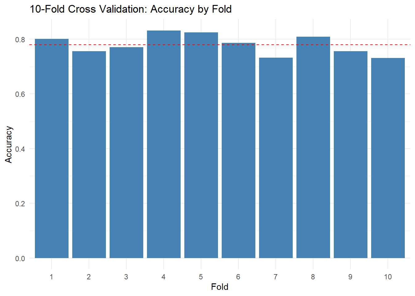
#> 0.780 0.036 0.731 0.8323.4 Visualize fold performance
It’s helpful to see how accuracy varies across folds. Create a simple bar chart or dot plot of the 10 fold accuracies. This visualization makes the variability concrete — you can see which folds were “easy” and which were “hard.”
Starter code
Click for a hint
Click for a solution
ggplot(cv_results, aes(x = factor(fold), y = accuracy)) +
  geom_col(fill = "steelblue") +
  geom_hline(yintercept = mean(cv_results$accuracy), linetype = "dashed", color = "red") +
  labs(
    title = "10-Fold Cross Validation: Accuracy by Fold",
    x = "Fold",
    y = "Accuracy"
  ) +
  theme_minimal()
Exercise 4: When the cutoff is a policy decision
A probability cutoff is not a law of nature. It is a decision.
Lloyd’s might treat “predict survival” as a proxy for “low risk,” but different cutoffs change what counts as low risk. A cutoff of 0.3 is generous: it labels many passengers as likely survivors, which could lead to under-pricing risk. A cutoff of 0.7 is conservative: it labels most passengers as non-survivors, which might over-price risk. The “right” cutoff depends on the costs of different errors — and those costs are a business decision, not a statistical one.
In this exercise you will examine how accuracy changes as the cutoff changes.
4.1 Evaluate multiple cutoffs on the test set
Using p_test from Exercise 2, compute test accuracy for the following cutoffs: 0.3, 0.5, 0.7.
Create a data frame called cutoff_results with columns cutoff and accuracy.
Starter code
Click for a hint
#>   cutoff accuracy
#> 1    0.3     0.70
#> 2    0.5     0.76
#> 3    0.7     0.79
Click for a solution
cutoffs <- c(0.3, 0.5, 0.7)

cutoff_results <- data.frame(
  cutoff = cutoffs,
  accuracy = NA_real_
)

for (i in seq_along(cutoffs)) {

  c0 <- cutoffs[i]

  yhat_c <- ifelse(p_test > c0, 1, 0)
  cutoff_results$accuracy[i] <- mean(yhat_c == titanic_test_survival$survived, na.rm = TRUE)

}

cutoff_results
#>   cutoff accuracy
#> 1    0.3     0.70
#> 2    0.5     0.76
#> 3    0.7     0.79
4.2 Visualize cutoff performance
To make the trade-off more concrete, let’s expand the analysis. Evaluate accuracy across a finer grid of cutoffs and plot the results. This will reveal that accuracy is not a smooth function of the cutoff — it can have a plateau or multiple peaks.
Starter code
Click for a hint

Click for a solution
cutoffs_fine <- seq(0.1, 0.9, by = 0.05)

cutoff_results_fine <- data.frame(
  cutoff = cutoffs_fine,
  accuracy = NA_real_
)

for (i in seq_along(cutoffs_fine)) {
  c0 <- cutoffs_fine[i]
  yhat_c <- ifelse(p_test > c0, 1, 0)
  cutoff_results_fine$accuracy[i] <- mean(yhat_c == titanic_test_survival$survived, na.rm = TRUE)
}

ggplot(cutoff_results_fine, aes(x = cutoff, y = accuracy)) +
  geom_line() +
  geom_point() +
  labs(
    title = "Test Accuracy Across Probability Cutoffs",
    x = "Cutoff",
    y = "Accuracy"
  ) +
  theme_minimal()
4.3 Reflection
- Which cutoff maximized accuracy here?
- Why might accuracy be a poor criterion for selecting a cutoff in underwriting? Think about what happens when the costs of false positives and false negatives differ.
- Name one alternative metric you would want if false positives and false negatives had different costs. (Hint: think about sensitivity, specificity, or expected cost.)
Stretch tasks (optional)
These are optional, but they bring the lab closer to how real modeling work looks. If you found the main exercises straightforward, these will push your understanding further.
5.1 Add one more predictor and re-run CV
Pick one additional predictor from titanic3 that you think should matter (for example, age or fare).
- Fit
survived ~ sex + pclass + <your variable>. - Run 10-fold CV again.
- Compare
cv_meanandcv_sdto the baseline model.
Important: decide how you will handle missing values for your added predictor (listwise deletion is allowed here; we will treat missingness more carefully in the super stretch exercises).
Starter code
titanic_cv51 <- titanic3 %>%
  filter(!is.na(___)) %>%
  filter(!is.na(___)) %>%
  filter(!is.na(___)) %>%
  filter(!is.na(___))

set.seed(42)
titanic_cv51 <- titanic_cv51 %>%
  mutate(fold = __________________ )

cv_results51 <- data.frame(fold =  ___________, accuracy =  ___________)
for (j in 1:10) {
  train_j <- titanic_cv51 %>% filter(fold != j)
  test_j  <- titanic_cv51 %>% filter(fold == j)
  m_j     <- glm( ___________, data =  ___________, family =  ___________)
  p_j     <- predict( ___________, newdata =  ___________, type = "response")
  yhat_j  <- ifelse( ___________ > 0.5, 1, 0)
  cv_results51$accuracy[j] <- mean(yhat_j ==  ___________, na.rm = TRUE)
}

c(cv_mean = mean(cv_results51$accuracy), cv_sd = sd(cv_results51$accuracy))
Click for a hint
You can reuse the CV loop from Exercise 3 with a new formula. Just make sure to filter out rows where your new predictor is missing before creating folds, so that every fold has the same set of variables available.
Click for a solution example
titanic_cv51 <- titanic3 %>%
  filter(!is.na(survived)) %>%
  filter(!is.na(sex)) %>%
  filter(!is.na(pclass)) %>%
  filter(!is.na(age))

set.seed(42)
titanic_cv51 <- titanic_cv51 %>%
  mutate(fold = sample(rep(1:10, length.out = n())))

cv_results51 <- data.frame(fold = 1:10, accuracy = NA_real_)
for (j in 1:10) {
  train_j <- titanic_cv51 %>% filter(fold != j)
  test_j  <- titanic_cv51 %>% filter(fold == j)
  m_j     <- glm(survived ~ sex + pclass + age, data = train_j, family = binomial)
  p_j     <- predict(m_j, newdata = test_j, type = "response")
  yhat_j  <- ifelse(p_j > 0.5, 1, 0)
  cv_results51$accuracy[j] <- mean(yhat_j == test_j$survived, na.rm = TRUE)
}

c(cv_mean = mean(cv_results51$accuracy), cv_sd = sd(cv_results51$accuracy))
#> cv_mean   cv_sd
#>   0.781   0.021
5.2 Competing models
Fit and compare at least two models using CV:
- Model A:
sex + pclass - Model B:
sex + pclass + <two more predictors>
Report which model has higher cv_mean. If the difference is small, argue which one you would recommend to Lloyd’s, considering simplicity vs performance. Remember that a simpler model is easier to explain to stakeholders and less likely to overfit.
Starter code
f_A <- survived ~ sex + pclass
f_B <- survived ~ sex + pclass + ___ + ___

cv_A <- _________(cv_df, formula = ___)
cv_B <- _________(cv_df, formula = ___)

data.frame(
  model   = c("A: base", "B: expanded"),
  cv_mean = c(mean(cv_A$accuracy), mean(cv_B$accuracy)),
  cv_sd   = c(sd(cv_A$accuracy),   sd(cv_B$accuracy))
)
Click for a hint
#> Error in `cv_glm_accuracy()`:
#> ! could not find function "cv_glm_accuracy"
#> Error in `cv_glm_accuracy()`:
#> ! could not find function "cv_glm_accuracy"
#> Error:
#> ! object 'cv_A' not found
Click for a solution example
f_A <- survived ~ sex + pclass
f_B <- survived ~ sex + pclass + age + fare

cv_A <- cv_glm_accuracy(cv_df, formula = f_A)
#> Error in `cv_glm_accuracy()`:
#> ! could not find function "cv_glm_accuracy"
cv_B <- cv_glm_accuracy(cv_df, formula = f_B)
#> Error in `cv_glm_accuracy()`:
#> ! could not find function "cv_glm_accuracy"

data.frame(
  model   = c("A: base", "B: expanded"),
  cv_mean = c(mean(cv_A$accuracy), mean(cv_B$accuracy)),
  cv_sd   = c(sd(cv_A$accuracy),   sd(cv_B$accuracy))
)
#> Error:
#> ! object 'cv_A' not found
5.3 Stability thought experiment
Repeat 10-fold CV but change the seed (try three different seeds). Does cv_mean change much? Does cv_sd change much?
Write 3 to 5 sentences interpreting what you see. If the results change a lot across seeds, what does that tell you about the reliability of your 10-fold estimate?
Super Stretch goals
Lloyd’s Actually Has to Use This Model
In the previous exercises, we evaluated a simple Titanic model using holdout testing and k-fold cross validation. That section began with a deliberately constrained model (sex and pclass) so you could focus on evaluation without getting lost in feature engineering.
Now we do the part Lloyd’s actually cares about: building a model that uses more information, and doing so in a way that does not quietly sabotage evaluation.
This section is about the uncomfortable truth that modeling choices are evaluation choices:
- If you add predictors with missing data, you change the population your model is trained and tested on.
- If you impute missing values using the full dataset, you leak information across folds.
- If you select a cutoff to maximize accuracy, you are making a policy decision without naming it.
You will build richer models, compare them using cross validation, and then stress-test the evaluation pipeline itself.
Additional Learning goals
- Compare multiple candidate models using k-fold cross validation.
- Handle missing data with listwise deletion and simple imputation.
- Avoid information leakage by imputing within folds.
- Evaluate classifiers beyond accuracy (confusion matrices, sensitivity/specificity).
- Reason about performance vs stability when recommending a model.
Exercise 6: Candidate models
Lloyd’s will not price risk using only sex and class. Your job is to propose reasonable candidate models and compare them using the same evaluation method. Think about what information an insurer would realistically have about a passenger before the voyage.
6.1 Choose candidate predictors
Pick two additional predictors from the data set. (This can include a constructed variable that you create from existing variables.)
names(titanic3)
#>  [1] "pclass"     "survived"   "name"       "sex"        "age"
#>  [6] "sibsp"      "parch"      "ticket"     "fare"       "cabin"
#> [11] "embarked"   "boat"       "body"       "home.dest"  "pclass_ord"
Why do you think each predictor you selected should matter for survival? Write a brief justification for each (2-3 sentences).
Click for a hint about feature engineering
Titles extracted from names (e.g., “Mr”, “Mrs”, “Miss”, “Master”) can be powerful predictors because they encode both sex and social status. Here’s how to extract them:
Click for a sample answer
Good candidate predictors include:
age: Children were prioritized during evacuation (“women and children first”), so younger passengers likely had higher survival rates. Age also correlates with physical ability to reach lifeboats.fare: Fare is a proxy for wealth and cabin location. Higher fares corresponded to upper-deck cabins closer to the lifeboats, giving wealthier passengers a structural advantage in evacuation.embarked: Port of embarkation (Cherbourg, Queenstown, Southampton) correlates with passenger demographics and class composition, which in turn predicts survival.
Exercise 7: Cross validation comparison (listwise deletion)
We will start with the simplest missing-data strategy: drop rows with missing values in any variable used by the model.
This is not always the best approach, but it is transparent and ensures that every row in the analysis has complete information. The cost is that we may lose a substantial number of passengers.
7.1 Create a CV dataset for both models
Create cv_df that keeps only rows with non-missing values for all variables needed in f_expanded. This way, both the baseline and expanded models are evaluated on the same set of passengers — an apples-to-apples comparison.
Click for a hint
7.3 Write a function to compute CV accuracy
In the main exercises, you wrote a for loop to perform cross validation. Now let’s wrap that logic into a reusable function. This is good programming practice: once you have code that works, encapsulating it in a function makes it easier to apply repeatedly and reduces the chance of copy-paste errors.
Complete the function below so it returns a data frame with fold accuracies for a given formula.
cv_glm_accuracy <- function(df, formula, cutoff = 0.5) {

  out <- data.frame(fold = sort(unique(df$fold)), accuracy = NA_real_)

  for (j in out$fold) {

    train_j <- df %>% filter(fold != ___)
    test_j  <- df %>% filter(fold == ___)

    m_j <- glm(
      formula = ___,
      data = ___,
      family = ___
    )

    p_j <- predict(m_j, newdata = ___, type = ___)
    yhat_j <- ifelse(___ > ___, ___, ___)

    out$accuracy[out$fold == j] <- mean(___ == ___, na.rm = TRUE)
  }

  out
}
Click for a hint
This function takes a data frame df with a fold variable, a model formula, and an optional cutoff. It loops through each fold, fits the specified logistic regression model on the training set, predicts on the test set, and computes accuracy based on the cutoff. The result is a data frame with fold-wise accuracies that can be summarized or compared across models.
Click for a solution
cv_glm_accuracy <- function(df, formula, cutoff = 0.5) {

  out <- data.frame(fold = sort(unique(df$fold)), accuracy = NA_real_)

  for (j in out$fold) {

    train_j <- df %>% filter(fold != j)
    test_j  <- df %>% filter(fold == j)

    m_j <- glm(
      formula = formula,
      data = train_j,
      family = binomial
    )

    p_j <- predict(m_j, newdata = test_j, type = "response")
    yhat_j <- ifelse(p_j > cutoff, 1, 0)

    out$accuracy[out$fold == j] <- mean(yhat_j == test_j$survived, na.rm = TRUE)
  }

  out
}
7.4 Compare models
Use cv_glm_accuracy() to compute CV results for both formulas. Compute mean and SD of accuracy for each.
Starter code
Click for a hint
#>      model mean_acc sd_acc
#> 1     base     0.78  0.039
#> 2 expanded     0.78  0.036
Click for a solution
cv_base <- cv_glm_accuracy(cv_df, formula = f_base)
cv_exp  <- cv_glm_accuracy(cv_df, formula = f_expanded)

summary_table <- data.frame(
  model = c("base", "expanded"),
  mean_acc = c(mean(cv_base$accuracy), mean(cv_exp$accuracy)),
  sd_acc   = c(sd(cv_base$accuracy), sd(cv_exp$accuracy))
)

summary_table
#>      model mean_acc sd_acc
#> 1     base     0.78  0.039
#> 2 expanded     0.78  0.036
7.5 Reflection
- Which model has higher mean CV accuracy?
- Which model has higher variability across folds?
- If the accuracy improvement is small but the expanded model is more variable, how would you advise Lloyd’s? Consider the trade-off between a slight improvement in average performance and greater uncertainty about how the model will perform on any given new passenger.
Exercise 8: Missingness is a modeling decision
Listwise deletion is convenient, but it changes your population: you are now modeling a subset of passengers with complete records on your chosen predictors. If the passengers with missing data differ systematically from those with complete data (for example, third-class passengers were less likely to have their ages recorded), your model may not generalize to the full population.
8.1 Quantify the missingness impact
Compute the number of rows in:
- the original
titanic3with non-missingsurvived cv_df
Report the proportion retained.
Starter code
Click for a hint
#>     n_all    n_kept prop_kept
#> 1309.0 1045.0 0.88.2 Investigate who is missing
Let’s dig deeper. Compare the survival rate and class distribution between passengers with complete data and those with missing age.
Starter code
Click for a hint
#> # A tibble: 2 × 5
#>   age_missing     n survival_rate pct_first_class pct_third_class
#>   <chr>       <int>         <dbl>           <dbl>           <dbl>
#> 1 Has age      1046         0.408           0.272           0.479
#> 2 Missing age   263         0.278           0.148           0.791
Click for a solution
titanic3 %>%
  filter(!is.na(survived)) %>%
  mutate(age_missing = ifelse(is.na(age), "Missing age", "Has age")) %>%
  group_by(age_missing) %>%
  summarize(
    n = n(),
    survival_rate = mean(survived, na.rm = TRUE),
    pct_first_class = mean(pclass == 1, na.rm = TRUE),
    pct_third_class = mean(pclass == 3, na.rm = TRUE)
  )
#> # A tibble: 2 × 5
#>   age_missing     n survival_rate pct_first_class pct_third_class
#>   <chr>       <int>         <dbl>           <dbl>           <dbl>
#> 1 Has age      1046         0.408           0.272           0.479
#> 2 Missing age   263         0.278           0.148           0.791
8.3 Reflection
- What kinds of passengers might be disproportionately removed by listwise deletion when you include
age? - Why does this matter for Lloyd’s, even if accuracy improves? (Hint: think about whether the model is being evaluated on a representative sample of the passengers Lloyd’s would actually insure.)
Exercise 9: Simple imputation without leakage
Now you will use a very simple imputation strategy for a numeric predictor:
- Replace missing values with the training-fold mean (not the overall mean).
This is the smallest step toward preventing leakage: the test fold should not influence how you fill in missing values. If you compute the mean on the full dataset and use it to fill in missing test-fold values, the test fold’s information has “leaked” into the imputation — your model has indirectly seen the test data.
9.1 Implement within-fold mean imputation for one variable
Choose one numeric predictor you used (for example, age). Complete the loop to:
- compute the mean of that variable in
train_j(excluding NAs), - fill missing values in both
train_jandtest_jusing that training mean, - fit the expanded model and compute fold accuracy.
Store results in cv_imp.
Starter code
cv_imp <- data.frame(fold = sort(unique(cv_df$fold)), accuracy = NA_real_)

for (j in cv_imp$fold) {

  train_j <- cv_df %>% filter(fold != ___)
  test_j  <- cv_df %>% filter(fold == ___)

  mu <- mean(train_j$___, na.rm = TRUE)

  train_j$___[is.na(train_j$___)] <- ___
  test_j$___[is.na(test_j$___)] <- ___

  m_j <- glm(
    formula = ___,
    data = ___,
    family = ___
  )

  p_j <- predict(m_j, newdata = ___, type = ___)
  yhat_j <- ifelse(___ > ___, ___, ___)

  cv_imp$accuracy[cv_imp$fold == j] <- mean(___ == ___, na.rm = TRUE)
}

c(mean = mean(cv_imp$accuracy), sd = sd(cv_imp$accuracy))
Click for a hint
#>  mean    sd
#> 0.777 0.036
Click for a solution example
cv_imp <- data.frame(fold = sort(unique(cv_df$fold)), accuracy = NA_real_)

for (j in cv_imp$fold) {

  train_j <- cv_df %>% filter(fold != j)
  test_j  <- cv_df %>% filter(fold == j)

  mu <- mean(train_j$age, na.rm = TRUE)

  train_j$age[is.na(train_j$age)] <- mu
  test_j$age[is.na(test_j$age)] <- mu

  m_j <- glm(
    formula = f_expanded,
    data = train_j,
    family = binomial
  )

  p_j <- predict(m_j, newdata = test_j, type = "response")
  yhat_j <- ifelse(p_j > 0.5, 1, 0)

  cv_imp$accuracy[cv_imp$fold == j] <- mean(yhat_j == test_j$survived, na.rm = TRUE)
}

c(mean = mean(cv_imp$accuracy), sd = sd(cv_imp$accuracy))
#>  mean    sd
#> 0.777 0.036
9.2 Reflection
- Why is imputing using the overall mean (computed on the full dataset) a form of leakage?
- Did within-fold imputation change mean CV accuracy compared to listwise deletion? Why might it?
- In practice, when might you want a more sophisticated imputation method than the mean? What are the trade-offs?
Exercise 10: Beyond accuracy (confusion matrix)
Accuracy treats all mistakes as equally bad. Lloyd’s rarely agrees. Predicting that a passenger survives when they actually perish (a false positive from the survival perspective) has very different financial implications than predicting they perish when they actually survive (a false negative).
A confusion matrix breaks predictions into four categories:
- True Positive (TP): Predicted survival, actually survived
- False Positive (FP): Predicted survival, actually perished
- True Negative (TN): Predicted non-survival, actually perished
- False Negative (FN): Predicted non-survival, actually survived
From these, we can compute:
- Sensitivity (True Positive Rate): TP / (TP + FN) — how well the model catches actual survivors
- Specificity (True Negative Rate): TN / (TN + FP) — how well the model identifies actual non-survivors
10.1 Compute confusion matrix elements on one fold
Pick a single fold (for example, fold 1). Using your chosen model and cutoff 0.5:
- compute TP, FP, TN, FN
- compute sensitivity and specificity
Starter code
# Choose a fold
j <- 1

train_j <- cv_df %>% filter(fold != j)
test_j  <- cv_df %>% filter(fold == j)

m_j <- glm(formula = f_expanded, data = __________, family = binomial)
p_j <- predict(m_j, newdata = __________, type = ___________)
yhat_j <- ifelse(p_j > 0.5, 1, 0)
y_j <- ________________

TP <- _____________
FP <- ___________
TN <- ___________
FN <- _____________

sensitivity <- _________ / (TP + FN)
specificity <- _______ / (TN + FP)

c(TP = TP, FP = FP, TN = TN, FN = FN, sensitivity = sensitivity, specificity = specificity)
Click for a hint
#>          TP          FP          TN          FN sensitivity specificity
#>       24.00       13.00       53.00       15.00        0.62        0.80
Click for a solution
j <- 1

train_j <- cv_df %>% filter(fold != j)
test_j  <- cv_df %>% filter(fold == j)

m_j <- glm(formula = f_expanded, data = train_j, family = binomial)
p_j <- predict(m_j, newdata = test_j, type = "response")
yhat_j <- ifelse(p_j > 0.5, 1, 0)
y_j <- test_j$survived

TP <- sum(yhat_j == 1 & y_j == 1, na.rm = TRUE)
FP <- sum(yhat_j == 1 & y_j == 0, na.rm = TRUE)
TN <- sum(yhat_j == 0 & y_j == 0, na.rm = TRUE)
FN <- sum(yhat_j == 0 & y_j == 1, na.rm = TRUE)

sensitivity <- TP / (TP + FN)
specificity <- TN / (TN + FP)

c(TP = TP, FP = FP, TN = TN, FN = FN, sensitivity = sensitivity, specificity = specificity)
#>          TP          FP          TN          FN sensitivity specificity
#>       24.00       13.00       53.00       15.00        0.62        0.80
10.2 Compute confusion metrics across all folds
Now extend this to all 10 folds. Store sensitivity and specificity for each fold alongside accuracy.
Starter code
cv_confusion <- data.frame(
  fold = sort(unique(cv_df$fold)),
  accuracy = NA_real_,
  sensitivity = NA_real_,
  specificity = NA_real_
)

for (j in cv_confusion$fold) {
  train_j <- cv_df %>% filter(fold != j)
  test_j  <- cv_df %>% filter(fold == j)

  m_j <- glm(formula = ___, data = ___, family = binomial)
  p_j <- predict(m_j, newdata = ___, type = "response")
  yhat_j <- ifelse(p_j > 0.5, 1, 0)
  y_j <- ______________________

  TP <- ___________
  FP <- ___________
  TN <- ___________
  FN <- ___________

  cv_confusion$accuracy[cv_confusion$fold == j] <- (TP + TN) / (___________)
  cv_confusion$sensitivity[cv_confusion$fold == j] <- TP / (___________)
  cv_confusion$specificity[cv_confusion$fold == j] <- TN / (___________)
}

cv_confusion
Click for a hint
#>    fold accuracy sensitivity specificity
#> 1     1     0.73        0.62        0.80
#> 2     2     0.84        0.79        0.86
#> 3     3     0.74        0.68        0.80
#> 4     4     0.78        0.67        0.86
#> 5     5     0.78        0.78        0.78
#> 6     6     0.76        0.70        0.80
#> 7     7     0.78        0.72        0.82
#> 8     8     0.75        0.63        0.87
#> 9     9     0.77        0.68        0.83
#> 10   10     0.84        0.71        0.95
Click for a solution
cv_confusion <- data.frame(
  fold = sort(unique(cv_df$fold)),
  accuracy = NA_real_,
  sensitivity = NA_real_,
  specificity = NA_real_
)

for (j in cv_confusion$fold) {
  train_j <- cv_df %>% filter(fold != j)
  test_j  <- cv_df %>% filter(fold == j)

  m_j <- glm(formula = f_expanded, data = train_j, family = binomial)
  p_j <- predict(m_j, newdata = test_j, type = "response")
  yhat_j <- ifelse(p_j > 0.5, 1, 0)
  y_j <- test_j$survived

  TP <- sum(yhat_j == 1 & y_j == 1, na.rm = TRUE)
  FP <- sum(yhat_j == 1 & y_j == 0, na.rm = TRUE)
  TN <- sum(yhat_j == 0 & y_j == 0, na.rm = TRUE)
  FN <- sum(yhat_j == 0 & y_j == 1, na.rm = TRUE)

  cv_confusion$accuracy[cv_confusion$fold == j] <- (TP + TN) / (TP + FP + TN + FN)
  cv_confusion$sensitivity[cv_confusion$fold == j] <- TP / (TP + FN)
  cv_confusion$specificity[cv_confusion$fold == j] <- TN / (TN + FP)
}

cv_confusion
#>    fold accuracy sensitivity specificity
#> 1     1     0.73        0.62        0.80
#> 2     2     0.84        0.79        0.86
#> 3     3     0.74        0.68        0.80
#> 4     4     0.78        0.67        0.86
#> 5     5     0.78        0.78        0.78
#> 6     6     0.76        0.70        0.80
#> 7     7     0.78        0.72        0.82
#> 8     8     0.75        0.63        0.87
#> 9     9     0.77        0.68        0.83
#> 10   10     0.84        0.71        0.95
10.3 Visualize the trade-off
Create a visualization that shows accuracy, sensitivity, and specificity side by side across folds. This will help you see whether the model is systematically better at catching one outcome than the other.
Starter code
cv_confusion_long <- cv_confusion %>%
  pivot_longer(cols = c(accuracy, sensitivity, specificity),
               names_to = "metric",
               values_to = "value")

ggplot(cv_confusion_long, aes(x = factor(fold), y = value, fill = metric)) +
  geom_col(position = "dodge") +
  labs(
    title = "Model Performance Across Folds",
    x = "Fold",
    y = "Value",
    fill = "Metric"
  ) +
  scale_fill_viridis_d() +
  theme_minimal()
Click for a hint
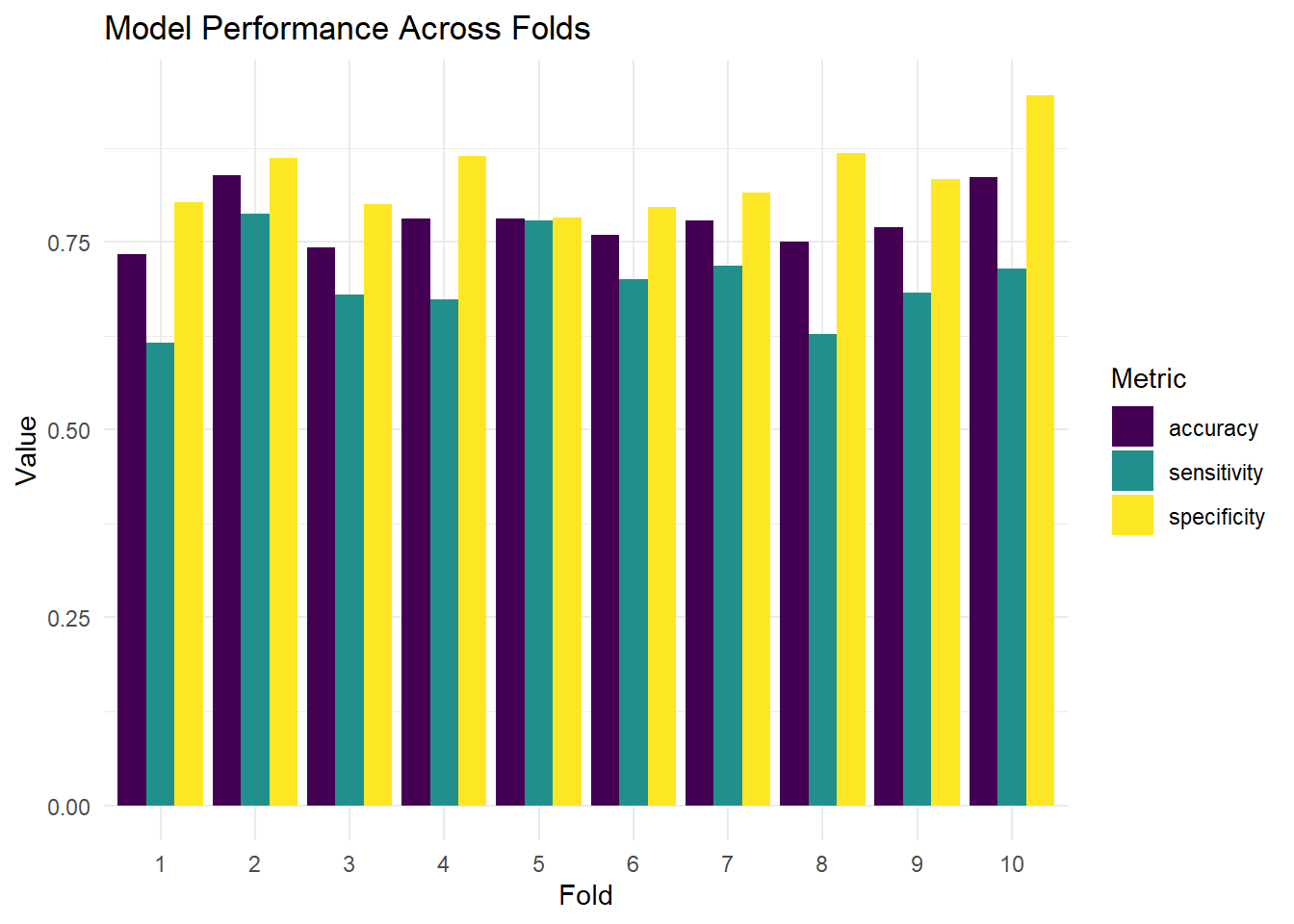
Click for a solution
cv_confusion_long <- cv_confusion %>%
  pivot_longer(cols = c(accuracy, sensitivity, specificity),
               names_to = "metric",
               values_to = "value")

ggplot(cv_confusion_long, aes(x = factor(fold), y = value, fill = metric)) +
  geom_col(position = "dodge") +
  labs(
    title = "Model Performance Across Folds",
    x = "Fold",
    y = "Value",
    fill = "Metric"
  ) +
  scale_fill_viridis_d() +
  theme_minimal()
10.4 Reflection
- Is the model better at identifying survivors (sensitivity) or non-survivors (specificity)?
- Which error type (FP or FN) would you expect to be more costly for Lloyd’s in a real risk context? Consider: a false positive means Lloyd’s predicts survival (low risk) for someone who actually perishes — that’s an under-priced policy. A false negative means Lloyd’s predicts non-survival (high risk) for someone who actually survives — that’s an over-priced policy that might lose the customer.
- How would that cost asymmetry change how you choose a cutoff?
- Given everything you’ve learned in this lab, write a brief recommendation (3-5 sentences) to Lloyd’s about how they should evaluate predictive models for maritime risk. What evaluation strategy would you recommend, and why?
Conclusion
Congratulations on completing the Cross Validation Lab! In this lab, you followed a progression that mirrors how real predictive modeling works:
- You started with apparent accuracy — the optimistic number you get when a model evaluates itself on its own training data.
- You moved to holdout testing — splitting the data into training and test sets to get a more honest estimate of performance.
- You implemented k-fold cross validation — repeating the train/test split across multiple folds to reduce dependence on any single partition.
- You explored how probability cutoffs change the meaning of a prediction and how that choice connects to real-world costs.
- In the stretch exercises, you encountered missingness, information leakage, and confusion matrices — the messy realities of building models that someone actually has to use.
Final Checklist
- Ensure you have completed and documented all exercises.
- Confirm that all code chunks execute without errors.
- Review your reflection answers — they should demonstrate understanding, not just correct code.
Reflect on Your Learning
- What was the most surprising thing you learned about model evaluation in this lab?
- How would you explain the difference between apparent accuracy and cross-validated accuracy to someone who has never taken a statistics course?
- If you were briefing Lloyd’s board of directors on your findings, what single takeaway would you emphasize?
Next Steps
- Commit all your changes to your project repository. Use a comprehensive commit message that reflects the completion of this lab.
- Push your changes to ensure everything is updated in your remote repository.
If you found this lab engaging, consider exploring the caret or tidymodels packages in R, which provide more streamlined tools for cross validation and model comparison. The concepts you learned here — honest evaluation, avoiding leakage, thinking about costs — apply no matter what tools you use.