68 Notes on Logistic Regression

68.1 Predicting categorical data

68.1.0.1 Spam filters

• Data from 3921 emails and 21 variables on them
• Outcome: whether the email is spam or not
• Predictors: number of characters, whether the email had “Re:” in the subject, time at which email was sent, number of times the word “inherit” shows up in the email, etc.

library(openintro)
data(email)
glimpse(email)
#> Rows: 3,921
#> Columns: 21
#> $ spam         <fct> 0, 0, 0, 0, 0, 0, 0, 0, 0, 0, 0, 0, 0, 0, 0, 0, 0, 0, 0, …
#> $ to_multiple  <fct> 0, 0, 0, 0, 0, 0, 1, 1, 0, 0, 0, 0, 0, 0, 0, 0, 0, 0, 0, …
#> $ from         <fct> 1, 1, 1, 1, 1, 1, 1, 1, 1, 1, 1, 1, 1, 1, 1, 1, 1, 1, 1, …
#> $ cc           <int> 0, 0, 0, 0, 0, 0, 0, 1, 0, 0, 0, 1, 0, 1, 2, 1, 0, 2, 0, …
#> $ sent_email   <fct> 0, 0, 0, 0, 0, 0, 1, 1, 0, 0, 1, 0, 0, 1, 0, 1, 0, 0, 1, …
#> $ time         <dttm> 2012-01-01 01:16:41, 2012-01-01 02:03:59, 2012-01-01 11:…
#> $ image        <dbl> 0, 0, 0, 0, 0, 0, 0, 1, 0, 0, 0, 0, 0, 0, 0, 0, 0, 0, 0, …
#> $ attach       <dbl> 0, 0, 0, 0, 0, 0, 0, 1, 0, 0, 0, 0, 0, 0, 0, 0, 0, 0, 0, …
#> $ dollar       <dbl> 0, 0, 4, 0, 0, 0, 0, 0, 0, 0, 0, 0, 0, 0, 2, 0, 5, 0, 0, …
#> $ winner       <fct> no, no, no, no, no, no, no, no, no, no, no, no, no, no, n…
#> $ inherit      <dbl> 0, 0, 1, 0, 0, 0, 0, 0, 0, 0, 0, 0, 0, 0, 0, 0, 0, 0, 0, …
#> $ viagra       <dbl> 0, 0, 0, 0, 0, 0, 0, 0, 0, 0, 0, 0, 0, 0, 0, 0, 0, 0, 0, …
#> $ password     <dbl> 0, 0, 0, 0, 2, 2, 0, 0, 0, 0, 0, 0, 0, 0, 0, 0, 1, 0, 0, …
#> $ num_char     <dbl> 11.370, 10.504, 7.773, 13.256, 1.231, 1.091, 4.837, 7.421…
#> $ line_breaks  <int> 202, 202, 192, 255, 29, 25, 193, 237, 69, 68, 25, 79, 191…
#> $ format       <fct> 1, 1, 1, 1, 0, 0, 1, 1, 0, 1, 1, 0, 1, 1, 1, 1, 1, 1, 0, …
#> $ re_subj      <fct> 0, 0, 0, 0, 0, 0, 0, 0, 0, 0, 0, 1, 0, 1, 1, 1, 0, 1, 1, …
#> $ exclaim_subj <dbl> 0, 0, 0, 0, 0, 0, 0, 0, 0, 0, 0, 0, 0, 0, 0, 0, 1, 0, 0, …
#> $ urgent_subj  <fct> 0, 0, 0, 0, 0, 0, 0, 0, 0, 0, 0, 0, 0, 0, 0, 0, 0, 0, 0, …
#> $ exclaim_mess <dbl> 0, 1, 6, 48, 1, 1, 1, 18, 1, 0, 2, 1, 0, 10, 4, 10, 20, 0…
#> $ number       <fct> big, small, small, small, none, none, big, small, small, …

Question: Would you expect longer or shorter emails to be spam?

#> Picking joint bandwidth of 1.18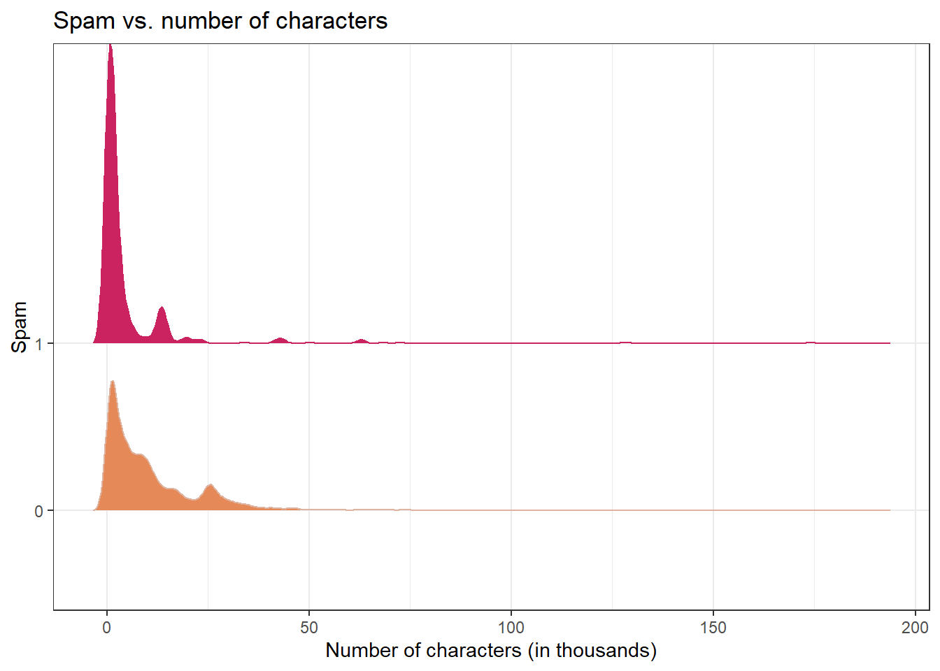

#> # A tibble: 2 × 2
#>   spam  mean_num_char
#>   <fct>         <dbl>
#> 1 0             11.3 
#> 2 1              5.44

Question: Would you expect emails that have subjects starting with “Re:”, “RE:”, “re:”, or “rE:” to be spam or not?

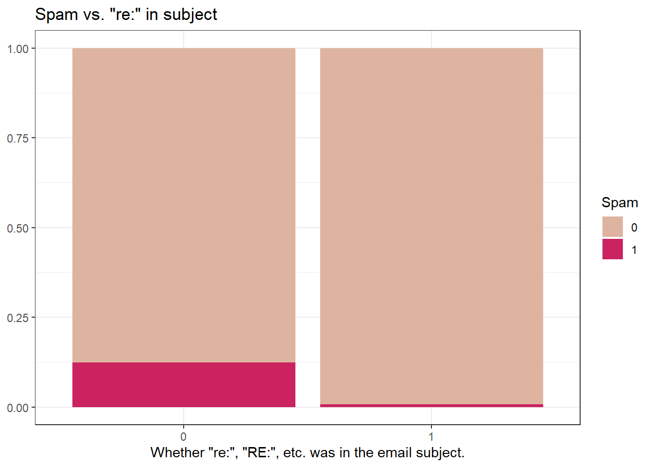
68.1.0.2 Modeling spam

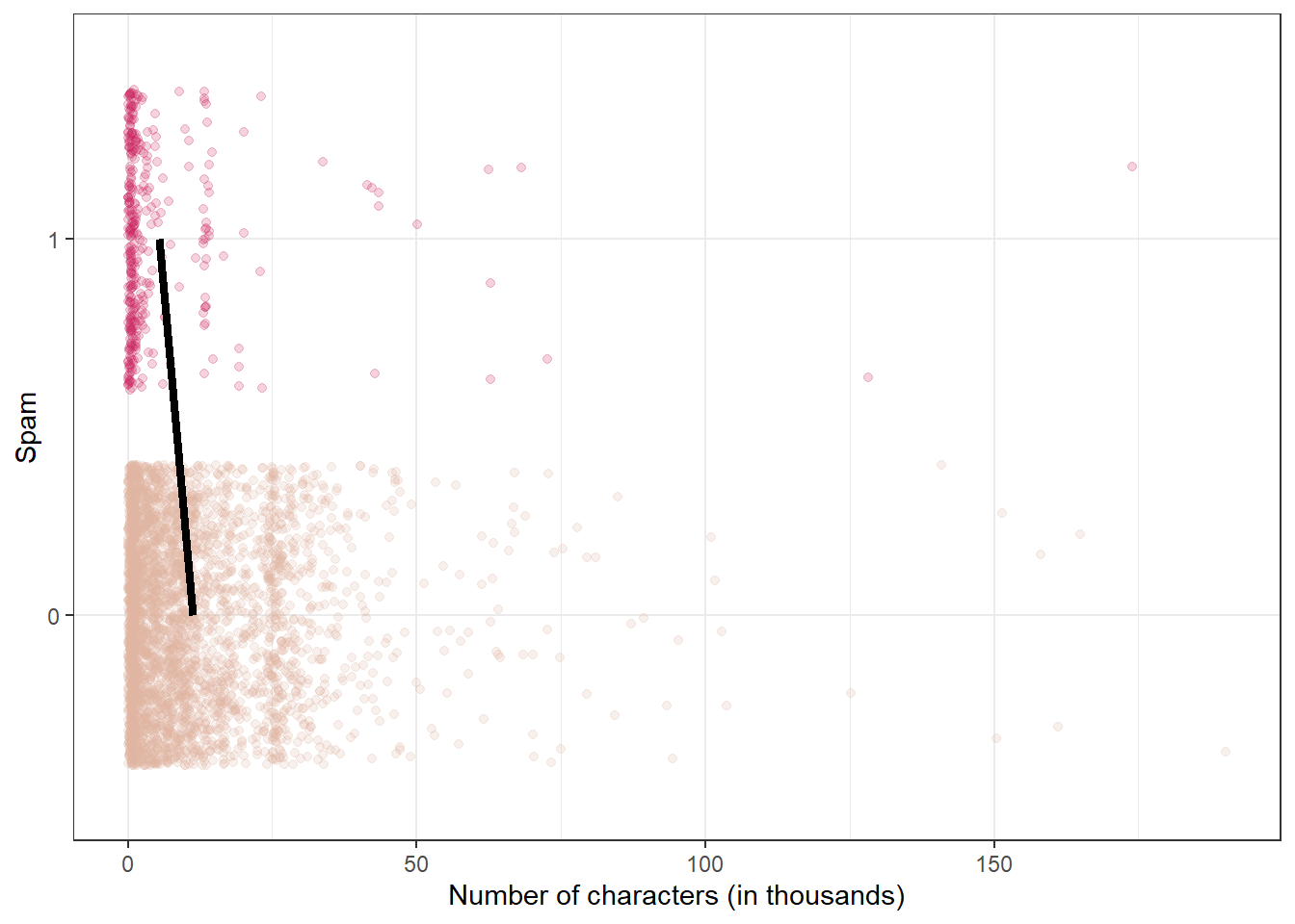
• Both number of characters and whether the message has “re:” in the subject might be related to whether the email is spam. How do we come up with a model that will let us explore this relationship?

• For simplicity, we’ll focus on the number of characters (num_char) as predictor, but the model we describe can be expanded to take multiple predictors as well.

We can’t reasonably fit a linear model to this data– we need something different!

68.1.0.3 Framing the problem

• We can treat each outcome (spam and not) as successes and failures arising from separate Bernoulli trials
  • Bernoulli trial: a random experiment with exactly two possible outcomes, “success” and “failure”, in which the probability of success is the same every time the experiment is conducted
• Each Bernoulli trial can have a separate probability of success

\[ y_i ∼ Bern(p) \]

• We can then use the predictor variables to model that probability of success, \(p_i\)

• We can’t just use a linear model for \(p_i\) (since \(p_i\) must be between 0 and 1) but we can transform the linear model to have the appropriate range

68.1.0.4 Generalized linear models

• This is a very general way of addressing many problems in regression and the resulting models are called generalized linear models (GLMs)

• Logistic regression is just one example

68.1.0.5 Three characteristics of GLMs

All GLMs have the following three characteristics:

1. A probability distribution describing a generative model for the outcome variable

2. A linear model: \[\eta = \beta_0 + \beta_1 X_1 + \cdots + \beta_k X_k\]

3. A link function that relates the linear model to the parameter of the outcome distribution

68.1.0.6 Logistic regression

• Logistic regression is a GLM used to model a binary categorical outcome using numerical and categorical predictors

• To finish specifying the Logistic model we just need to define a reasonable link function that connects \(\eta_i\) to \(p_i\): logit function

• Logit function: For \(0\le p \le 1\)

\[logit(p) = \log\left(\frac{p}{1-p}\right)\]

68.1.0.7 Logit function, visualized

d <- tibble(p = seq(0.001, 0.999,
  length.out = 1000
)) %>%
  mutate(logit_p = log(p / (1 - p)))

ggplot(d, aes(x = p, y = logit_p)) +
  geom_line() +
  xlim(0, 1) +
  ylab("logit(p)") +
  labs(title = "logit(p) vs. p") + theme_bw()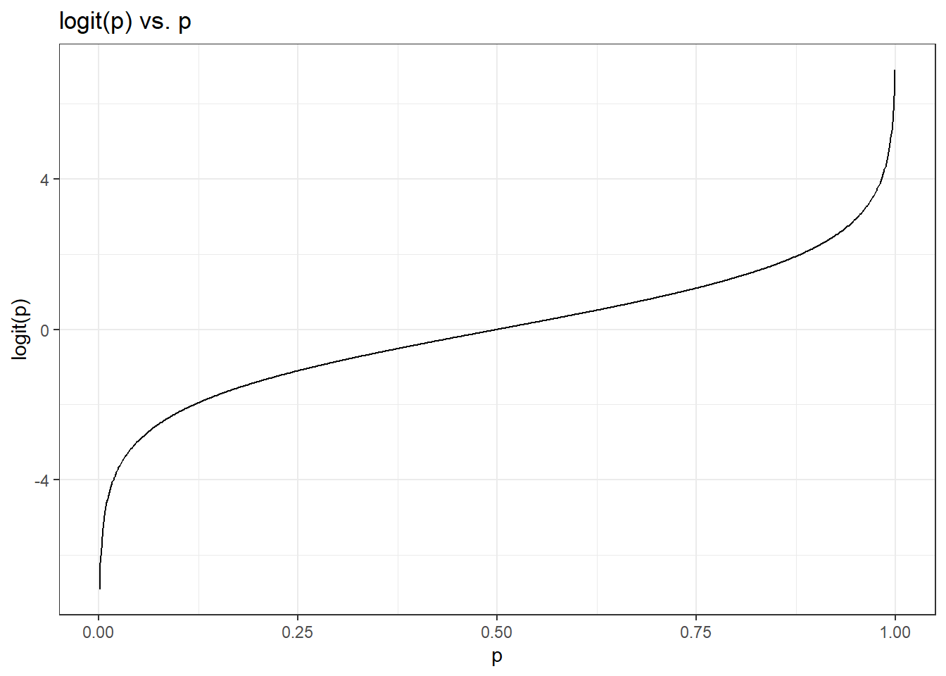

68.1.0.8 Properties of the logit

• The logit function takes a value between 0 and 1 and maps it to a value between \(-\infty\) and \(\infty\)

• Inverse logit (logistic) function: \[g^{-1}(x) = \frac{\exp(x)}{1+\exp(x)} = \frac{1}{1+\exp(-x)}\]

• The inverse logit function takes a value between \(-\infty\) and \(\infty\) and maps it to a value between 0 and 1

• This formulation is also useful for interpreting the model, since the logit can be interpreted as the log odds of a success – more on this later

68.1.0.9 The logistic regression model

• Based on the three GLM criteria, we have
  • \(y_i \sim \text{Bern}(p_i)\)
  • \(\eta_i = \beta_0+\beta_1 x_{1,i} + \cdots + \beta_n x_{n,i}\)
  • \(\text{logit}(p_i) = \eta_i\)
• From which we get

\[p_i = \frac{\exp(\beta_0+\beta_1 x_{1,i} + \cdots + \beta_k x_{k,i})}{1+\exp(\beta_0+\beta_1 x_{1,i} + \cdots + \beta_k x_{k,i})}\]

68.1.0.10 Modeling spam

In R, we fit a GLM in the same way as a linear model except we

• specify the model with logistic_reg()
• use "glm" instead of "lm" as the engine
• define family = "binomial" for the link function to be used in the model

spam_fit <- logistic_reg() %>%
  set_engine("glm") %>%
  fit(spam ~ num_char,
    data = email,
    family = "binomial"
  )

# tidy(spam_fit)

68.1.0.11 Spam model

tidy(spam_fit)
#> # A tibble: 2 × 5
#>   term        estimate std.error statistic   p.value
#>   <chr>          <dbl>     <dbl>     <dbl>     <dbl>
#> 1 (Intercept)  -1.80     0.0716     -25.1  2.04e-139
#> 2 num_char     -0.0621   0.00801     -7.75 9.50e- 15

Model: \[\log\left(\frac{p}{1-p}\right) = -1.80-0.0621\times \text{num_char}\]

68.1.0.12 P(spam) for an email with 2000 characters

\[\log\left(\frac{p}{1-p}\right) = -1.80-0.0621\times 2\]

\[\frac{p}{1-p} = \exp(-1.9242) = 0.15 \rightarrow p = 0.15 \times (1 - p)\]

\[p = 0.15 - 0.15p \rightarrow 1.15p = 0.15\]

\[p = 0.15 / 1.15 = 0.13\]

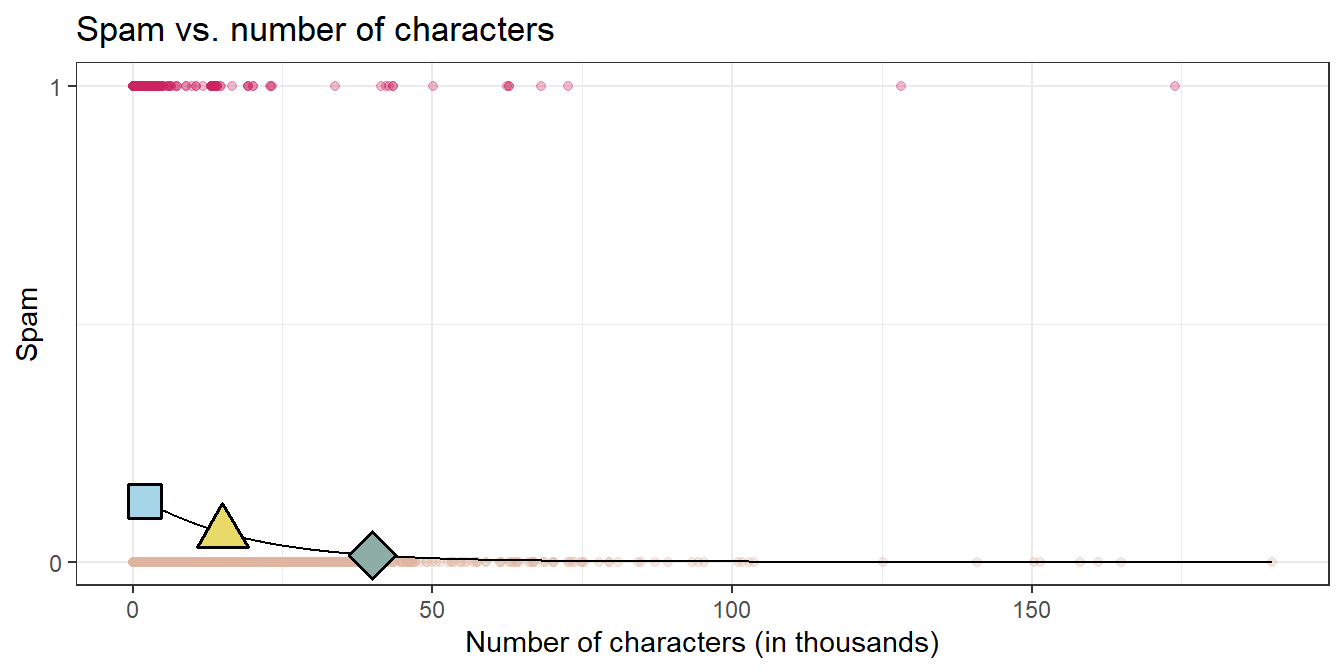
Question: What is the probability that an email with 15000 characters is spam? What about an email with 40000 characters?

• 2K chars: P(spam) = 0.13
• 15K chars, P(spam) = 0.06
• 40K chars, P(spam) = 0.01

Question: Would you prefer an email with 2000 characters to be labeled as spam or not? How about 40,000 characters?

68.2 Sensitivity and specificity

68.2.0.1 False positive and negative

	Email is spam	Email is not spam
Email labeled spam	True positive	False positive (Type 1 error)
Email labeled not spam	False negative (Type 2 error)	True negative

• False negative rate = P(Labeled not spam | Email spam) = FN / (TP + FN)

• False positive rate = P(Labeled spam | Email not spam) = FP / (FP + TN)

68.2.0.2 Sensitivity and specificity

	Email is spam	Email is not spam
Email labeled spam	True positive	False positive (Type 1 error)
Email labeled not spam	False negative (Type 2 error)	True negative

• Sensitivity = P(Labeled spam | Email spam) = TP / (TP + FN)
  • Sensitivity = 1 − False negative rate
• Specificity = P(Labeled not spam | Email not spam) = TN / (FP + TN)
  • Specificity = 1 − False positive rate

Question: If you were designing a spam filter, would you want sensitivity and specificity to be high or low? What are the trade-offs associated with each decision?