60 LEC: Use API-wrapping packages
You can follow along with the slides here if you would like to open them full-screen.
60.1 ODD: Demystifying APIs with R Wrappers
This section explores how to use R packages that wrap APIs, allowing easy access to web data. We’ll cover various approaches from simple downloads to more complex API interactions. This content builds on Jenny Bryan’s stat545 materials, with significant updates and additions to reflect current best practices. For a more in-depth look at APIs, check out the API chapter in the R for Data Science book. For a huge list of free apis to play with, check out this list
Google trends analytics is helpful in the study of global web search patterns.
— R Function A Day (@rfunctionaday) April 13, 2021
The {gtrends} function from {gtrendsR} 📦 helps extract and visualize this data for specified periods and geolocations 🔎https://t.co/yS01ELq5q4#rstats #DataScience pic.twitter.com/mhGTSXB2rN
60.2 The Data Acquisition Spectrum
When it comes to obtaining data from the internet, we can categorize methods into four main type * Direct Download: Grabbing readily available flat files (CSV, XLS, etc.) * Wrapped API Access: Using R packages designed for specific APIs * Raw API Interaction: Crafting custom queries for APIs * Web Scraping: Extracting data embedded in HTML structures
We’ll focus primarily on the second method, but now you know about the full spectrum of options at your disposal. For a comprehensive list of R tools for interacting with the internet, check out the rOpenSci repository. These tools include packages for APIs, scraping, and more.
60.2.1 Direct Download
In the simplest case, the data you need is already on the internet in a tabular format. Effectively, you just need to click and download whatever data you need. There are a couple of strategies here:
- Use
read.csvorreadr::read_csvto read the data straight into R. - Use the command line program
curlto do that work, and place it in aMakefileor shell script (see the section onmakefor more on this).
The second case is most useful when the data you want has been provided in a format that needs cleanup. For example, the World Value Survey makes several datasets available as Excel sheets. The safest option here is to download the .xls file, then read it into R with readxl::read_excel() or something similar. An exception to this is data provided as Google Spreadsheets, which can be read straight into R using the googlesheets package.
60.2.1.1 From rOpenSci web services page
From rOpenSci’s CRAN Task View: Web Technologies and Services:
downloader::download()for SSL.curl::curl()for SSL.httr::GETdata read this way needs to be parsed later withread.table().rio::import()can “read a number of common data formats directly from anhttps://URL”. Isn’t that very similar to the previous?
What about packages that install data?
60.2.2 Data supplied on the web
Many times, the data that you want is not already organized into one or a few tables that you can read directly into R. More frequently, you find this data is given in the form of an API. Application Programming Interfaces (APIs) are descriptions of the kind of requests that can be made of a certain piece of software, and descriptions of the kind of answers that are returned.
Many sources of data – databases, websites, services – have made all (or part) of their data available via APIs over the internet. Computer programs (“clients”) can make requests of the server, and the server will respond by sending data (or an error message). This client can be many kinds of other programs or websites, including R running from your laptop.
60.2.3 Streamlined Data Retrieval with API Wrappers
Many common web services and APIs have been “wrapped”, i.e. R functions have been written around them which send your query to the server and format the response. This is a great way to get started with APIs, as you don’t need to worry about the details of the API itself. You can just focus on the data you want to get.
API-wrapping packages act as intermediaries between your R environment and web services. They handle the nitty-gritty of API calls, authentication, and data parsing, allowing you to focus on analysis rather than data acquisition logistics. These packages are especially useful for beginners, as they abstract away the complexities of web service interaction. For added bonuses, they often ensure that the data you receive is actually from the API you intended to query, and they provide a structured reproducible way to access the data.
60.2.3.1 Case Study: Ornithological Data with rebird
Let’s dive into a practical example using the rebird package, which interfaces with the eBird database. eBird lets birders upload sightings of birds, and allows everyone access to those data. rebird makes it easy to access this data from R (as long as you request an API key)
First, let’s fetch recent bird sightings from a specific location:
60.2.3.1.1 Search birds by geography
The eBird website categorizes some popular locations as “Hotspots”. These are areas where there are both lots of birds and lots of birders. One such location is at Iona Island, near Vancouver. You can see data for this Hotspot at http://ebird.org/ebird/hotspot/L261851.
At that link, you will see a page like this:
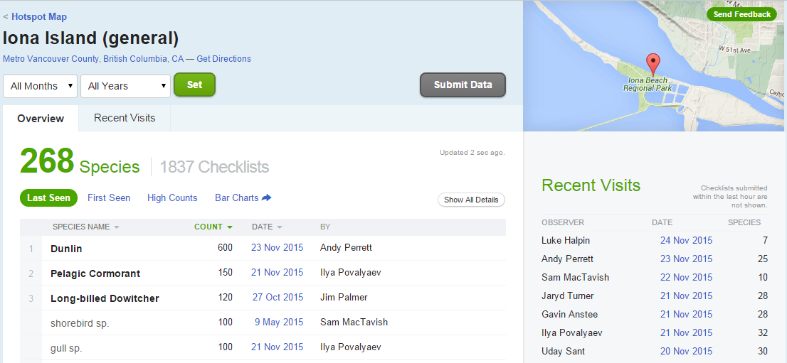
Figure 60.1: Iona Island
The data already looks to be organized in a data frame! rebird allows us to read these data directly into R (the ID code for Iona Island is “L261851”). Note that this requires an API key which you have to request from ebird via this link . I have set my key as an environment variable. However you can set it as a global variable in your R session. Like this:
ebirdregion(loc = "L261851", key = ebirdkey) %>%
  head() %>%
  kable()
#> Error in `curl::curl_fetch_memory()`:
#> ! Timeout was reached [ebird.org]:
#> Connection timed out after 10002 milliseconds
We can use the function ebirdgeo() to get a list for an area (note that South and West are negative):
vanbirds <- ebirdgeo(lat = 49.2500, lng = -123.1000, key = ebirdkey)
vanbirds %>%
  head() %>%
kable()| speciesCode | comName | sciName | locId | locName | obsDt | howMany | lat | lng | obsValid | obsReviewed | locationPrivate | subId | exoticCategory |
|---|---|---|---|---|---|---|---|---|---|---|---|---|---|
| cangoo | Canada Goose | Branta canadensis | L7942626 | Vancouver Convention Centre | 2026-05-08 00:13 | 2 | 49.3 | -123 | TRUE | FALSE | FALSE | S334360097 | NA |
| glwgul | Glaucous-winged Gull | Larus glaucescens | L7942626 | Vancouver Convention Centre | 2026-05-08 00:13 | 5 | 49.3 | -123 | TRUE | FALSE | FALSE | S334360097 | NA |
| buwtea | Blue-winged Teal | Spatula discors | L8204510 | Charleson Park & Seawall | 2026-05-07 20:34 | 1 | 49.3 | -123 | TRUE | FALSE | FALSE | S334324410 | NA |
| cintea | Cinnamon Teal | Spatula cyanoptera | L8204510 | Charleson Park & Seawall | 2026-05-07 20:34 | 1 | 49.3 | -123 | TRUE | FALSE | FALSE | S334324410 | NA |
| mallar3 | Mallard | Anas platyrhynchos | L58333621 | Vancouver — Cardero Park | 2026-05-07 19:48 | 1 | 49.3 | -123 | TRUE | FALSE | FALSE | S334321023 | NA |
| annhum | Anna’s Hummingbird | Calypte anna | L58333621 | Vancouver — Cardero Park | 2026-05-07 19:48 | 2 | 49.3 | -123 | TRUE | FALSE | FALSE | S334321023 | NA |
Note: Check the defaults on this function (e.g. radius of circle, time of year).
We can also search by “region”, which refers to short codes which serve as common shorthands for different political units. For example, France is represented by the letters FR.
| speciesCode | comName | sciName | locId | locName | obsDt | howMany | lat | lng | obsValid | obsReviewed | locationPrivate | subId | exoticCategory |
|---|---|---|---|---|---|---|---|---|---|---|---|---|---|
| blkswa | Black Swan | Cygnus atratus | L5556319 | Ile de Noirmoutier–Station d’épuration la Salaisière | 2026-05-08 13:51 | 1 | 47.0 | -2.26 | TRUE | FALSE | FALSE | S334453390 | X |
| litegr | Little Egret | Egretta garzetta | L5556319 | Ile de Noirmoutier–Station d’épuration la Salaisière | 2026-05-08 13:51 | 4 | 47.0 | -2.26 | TRUE | FALSE | FALSE | S334453390 | NA |
| mutswa | Mute Swan | Cygnus olor | L5556319 | Ile de Noirmoutier–Station d’épuration la Salaisière | 2026-05-08 13:51 | 4 | 47.0 | -2.26 | TRUE | FALSE | FALSE | S334453390 | NA |
| mallar3 | Mallard | Anas platyrhynchos | L5556319 | Ile de Noirmoutier–Station d’épuration la Salaisière | 2026-05-08 13:51 | 4 | 47.0 | -2.26 | TRUE | FALSE | FALSE | S334453390 | NA |
| comhom1 | Western House-Martin | Delichon urbicum | L65346332 | Hunawihr | 2026-05-08 13:45 | NA | 48.2 | 7.31 | TRUE | FALSE | TRUE | S334453041 | NA |
| combuz1 | Common Buzzard | Buteo buteo | L65346332 | Hunawihr | 2026-05-08 13:45 | 1 | 48.2 | 7.31 | TRUE | FALSE | TRUE | S334453041 | NA |
Find out when a bird has been seen in a certain place! Choosing a name from vanbirds above (the Bald Eagle):
eagle <- ebirdgeo(
  species = "baleag",
  lat = 42, lng = -76, key = ebirdkey
)
eagle %>%
  head() %>%
kable()| speciesCode | comName | sciName | locId | locName | obsDt | howMany | lat | lng | obsValid | obsReviewed | locationPrivate | subId |
|---|---|---|---|---|---|---|---|---|---|---|---|---|
| baleag | Bald Eagle | Haliaeetus leucocephalus | L8882294 | Nowlan Road | 2026-05-07 15:00 | 1 | 42.1 | -75.9 | TRUE | FALSE | TRUE | S334247860 |
| baleag | Bald Eagle | Haliaeetus leucocephalus | L65272841 | I-81 S, Binghamton US-NY 42.10830, -75.84226 | 2026-05-07 12:30 | 2 | 42.1 | -75.8 | TRUE | FALSE | TRUE | S334099726 |
| baleag | Bald Eagle | Haliaeetus leucocephalus | L65305656 | I-81 S, Binghamton US-NY 42.20387, -75.89909 | 2026-05-07 12:19 | 1 | 42.2 | -75.9 | TRUE | FALSE | TRUE | S334255645 |
| baleag | Bald Eagle | Haliaeetus leucocephalus | L1005329 | Brick Pond Wetland Preserve | 2026-05-06 17:45 | 1 | 42.1 | -76.2 | TRUE | FALSE | FALSE | S333931756 |
| baleag | Bald Eagle | Haliaeetus leucocephalus | L18141052 | Beer tree, Rt 369, Broome | 2026-05-05 16:09 | 1 | 42.2 | -75.8 | TRUE | FALSE | TRUE | S333206746 |
| baleag | Bald Eagle | Haliaeetus leucocephalus | L505437 | Boland Pond | 2026-05-03 15:30 | 1 | 42.2 | -75.9 | TRUE | FALSE | FALSE | S332091786 |
rebird knows where you are:
ebirdgeo(species = "rolhaw", key = ebirdkey)
#> Warning: As a complete lat/long pair was not provided, your location was
#> determined using your computer's public-facing IP address. This will likely not
#> reflect your physical location if you are using a remote server or proxy.
#> # A tibble: 0 × 0
60.2.3.2 Case Study: Searching geographic info: geonames
rOpenSci has a package called geonames for accessing the GeoNames API. First, install the geonames package from CRAN and load it.
The geonames package website tells us that there are a few things we need to do before we can use geonames to access the GeoNames API:
- Go to the GeoNames site and create a new user account.
- Check your email and follow the instructions to activate your account.
- You have to manually enable the free web services for your account (Note! You must be logged into your GeoNames account).
- Tell R your GeoNames username.
To do the last step, we could run this line in R…
…but this is insecure. We don’t want to risk committing this line and pushing it to our public GitHub page!
Instead, we can add this line to our .Rprofile so it will be hidden. One way to edit your .Rprofile is with the helper function edit_r_profile() from the usethis package. Install/load the usethis package and run edit_r_profile() in the R Console:
This will open up your .Rprofile file. Add options(geonamesUsername="my_user_name") on a new line (replace “my_user_name” with your GeoNames username).
Important: Make sure your .Rprofile ends with a blank line!
Save the file, close it, and restart R. Now we’re ready to start using geonames to search the GeoNames API.
(Also see the Cache credentials for HTTPS chapter of Happy Git and GitHub for the useR.)
60.2.3.2.1 Using GeoNames
What can we do? We can get access to lots of geographical information via the various GeoNames WebServices.
This countryInfo dataset is very helpful for accessing the rest of the data because it gives us the standardized codes for country and language.
60.2.3.3 Wikipedia searching
We can use geonames to search for georeferenced Wikipedia articles. Here are those within 20 km of Rio de Janerio, comparing results for English-language Wikipedia (lang = "en") and Portuguese-language Wikipedia (lang = "pt"):
60.2.4 Case Study: Is it a boy or a girl? Gender-associated names throughout US history
The gender package allows you access to data on the gender of names in the US. Because names change gender over the years, the probability of a name belonging to a man or a woman also depends on the year.
First, install/load the gender package from CRAN. You may be prompted to also install the companion package, genderdata. Go ahead and say yes. If you don’t see this message no need to worry, it is a one-time install.
# install.packages("gender")
if (!require(genderdata)) {
  remotes::install_github("lmullen/genderdata")
}
#> Loading required package: genderdata
if (!require(genderdata)) {
  genderdata_available <- FALSE
} else {
  genderdata_available <- TRUE
}
library(gender)
Let’s do some searches for the name Kelsey.
gender("Kelsey")
#> # A tibble: 1 × 6
#>   name   proportion_male proportion_female gender year_min year_max
#>   <chr>            <dbl>             <dbl> <chr>     <dbl>    <dbl>
#> 1 Kelsey          0.0314             0.969 female     1932     2012
gender("Kelsey", years = 1940)
#> # A tibble: 1 × 6
#>   name   proportion_male proportion_female gender year_min year_max
#>   <chr>            <dbl>             <dbl> <chr>     <dbl>    <dbl>
#> 1 Kelsey               1                 0 male       1940     1940
As you can see, the probability of a name belonging to a specific gender can change over time.
df <- gender("Kelsey")

years <- c(df$year_min:df$year_max)

for (i in 1:length(years)) {
  df <- rbind(df, gender("Kelsey", years = years[i]))
}
df %>%
  filter(year_min == year_max) %>%
  ggplot(aes(year_min, proportion_male)) +
  geom_smooth(span = 0.1) +
  labs(
    title = "Proportion of men named Kelsey over time",
    x = "Year",
    y = "Proporiton Male"
  ) +
  ggthemes::theme_excel()
#> `geom_smooth()` using method = 'loess' and formula = 'y ~ x'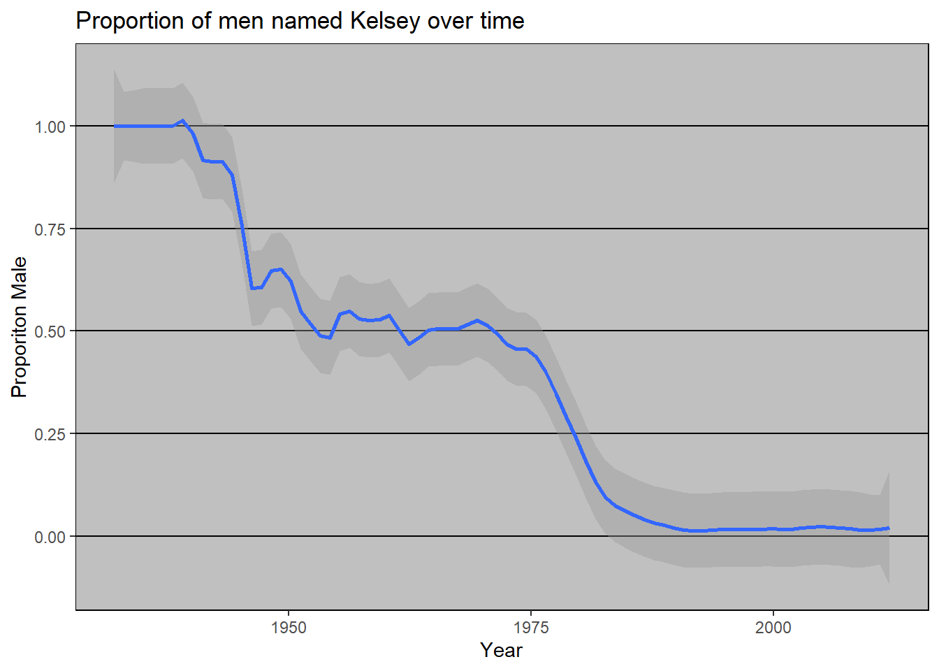
In contrast, the name Mason has been more consistently male.
gender("Mason")
#> # A tibble: 1 × 6
#>   name  proportion_male proportion_female gender year_min year_max
#>   <chr>           <dbl>             <dbl> <chr>     <dbl>    <dbl>
#> 1 Mason           0.987            0.0134 male       1932     2012
gender("Mason", years = 1940)
#> # A tibble: 1 × 6
#>   name  proportion_male proportion_female gender year_min year_max
#>   <chr>           <dbl>             <dbl> <chr>     <dbl>    <dbl>
#> 1 Mason               1                 0 male       1940     1940
mason <- gender("Mason")
years <- c(mason$year_min:mason$year_max)
df <- rbind(df, gender("Mason"))
for (i in 1:length(years)) {
df <- rbind(df, gender("Mason", years = years[i]))
}
df %>%
filter(year_min == year_max & name == "Mason") %>%
ggplot(aes(year_min, proportion_male)) +
geom_point() +
geom_smooth(span = 0.1) +
labs(
title = "Proportion of men named Mason over time",
x = "Year",
y = "Proporiton Male"
) +
ggthemes::theme_excel()
#> `geom_smooth()` using method = 'loess' and formula = 'y ~ x'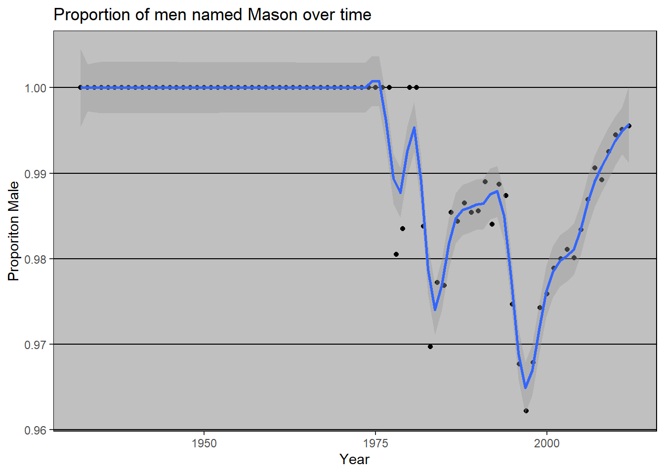
And when we compare the two names, we see that Kelsey has changed a lot more over time than Mason.
df %>%
  filter(year_min == year_max) %>%
  ggplot(aes(year_min, proportion_male)) +
  geom_point() +
  geom_smooth(span = 0.1) +
  labs(
    title = "Proportion of men over time",
    x = "Year",
    y = "Proporiton Male"
  ) +
  ggthemes::theme_excel() +
  facet_wrap(~name)
#> `geom_smooth()` using method = 'loess' and formula = 'y ~ x'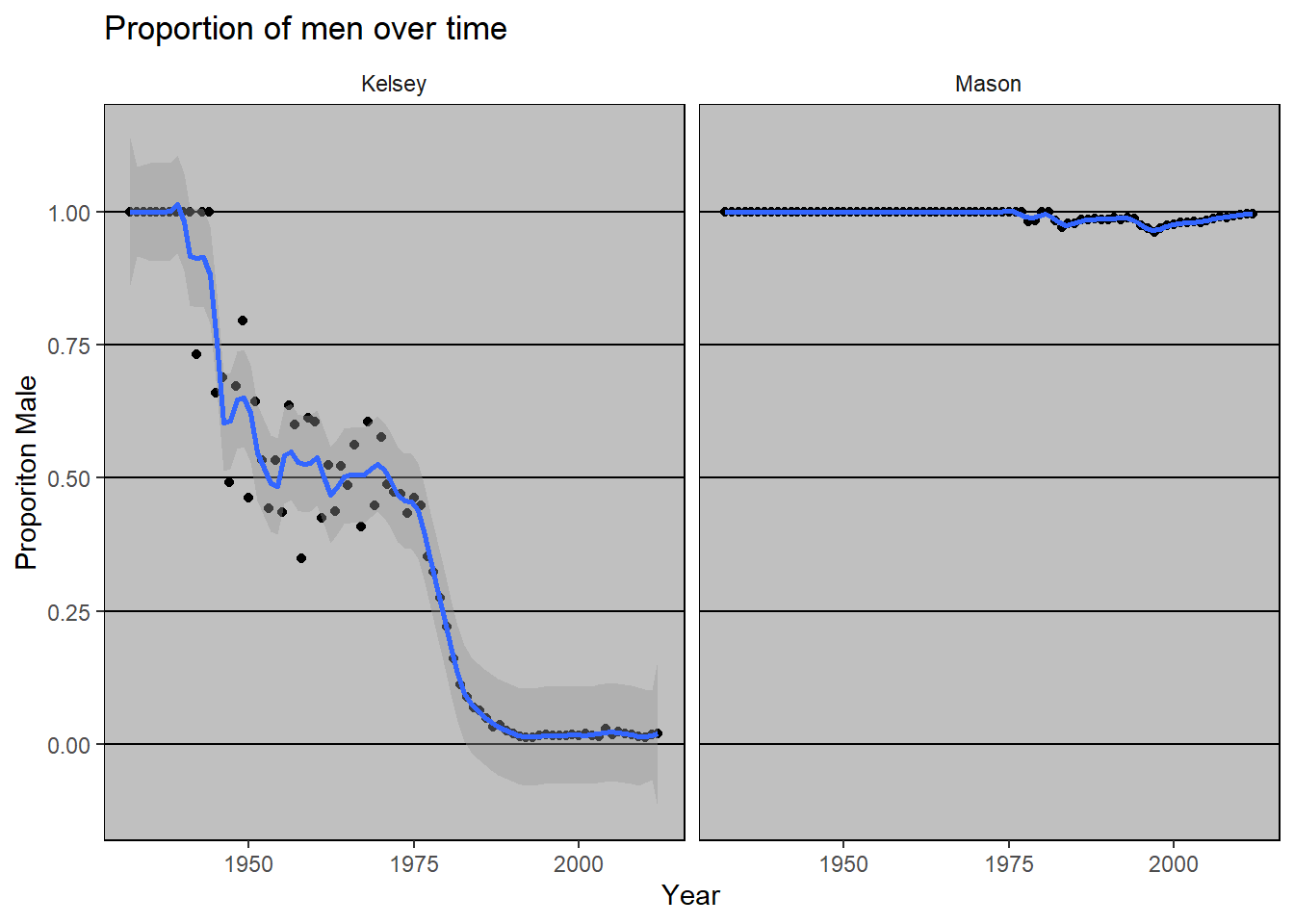
60.3 Conclusion
API-wrapping packages in R provide powerful tools for accessing diverse data sources. As you progress in your data science journey, mastering these tools will greatly expand the range of data available for your analyses. Remember to always check the terms of service for any API you use, and be mindful of rate limits and data usage policies.