42 LAB: Visualizing spatial data
La Quinta is Spanish for ‘next to Denny’s’, Pt. 1

Have you ever taken a road trip in the US and thought to yourself “I wonder what La Quinta means”. Well, the late comedian Mitch Hedberg has joked that it’s Spanish for next to Denny’s.
If you’re not familiar with these two establishments, Denny’s is a casual diner chain that is open 24 hours and La Quinta Inn and Suites is a hotel chain. In the US, diners and mid-range chain hotels are common along interstate highways. It’s typical to see clusters of brands near highway exits where travelers stop for food and lodging.
These two establishments tend to be clustered together, or at least this observation is a joke made famous by Mitch Hedberg. In this lab, we explore the validity of this joke and along the way learn some more data wrangling and tips for visualizing spatial data.
This lab was inspired by John Reiser’s post in his New Jersey geographer blog. You can read that analysis here. Reiser’s blog post focuses on scraping data from Denny’s and La Quinta Inn and Suites websites using Python. In this lab, we focus on visualization and analysis of those data. However, it’s worth noting that the data scraping was also done in R. Later in the course,we will discuss web scraping using R . But for now, we’re focusing on the data that has already been scraped and tidied up for you.
Getting started
Go to the course GitHub organization and locate the lab repo, which should be named something like lab-04-viz-sp-data. This link should take you to the lab. Either Fork it or use the template. Then clone it in RStudio. First, open the R Markdown document lab-04.Rmd and Knit it. Make sure it compiles without errors. The output will be in the file markdown .md file with the same name.
Packages
In this lab, we will use the tidyverse and dsbox packages. The dsbox package is currently not available on CRAN. However, you can find the most current version hosted on GitHub. Therefore, you will need to download and install it yourself. This piece of code should help get you started.
If you run into issues installing the dsbox package, don’t worry! You can still complete the lab by downloading the datasets directly from GitHub. The code below will load the two datasets we will be using directly from GitHub.Click to expand alternative data loading instructions
If you cannot get dsbox to install, you can instead download the two datasets we will be using manually here and here. You will need to save them in the data folder of your lab.
githubURL_lq <- "https://github.com/DataScience4Psych/DataScience4Psych/raw/main/data/raw/laquinta.csv"

githubURL_dn <- "https://github.com/DataScience4Psych/DataScience4Psych/raw/main/data/raw/dennys.csv"


laquinta <- readr::read_csv(githubURL_lq)
dennys <-   readr::read_csv(githubURL_dn)
Project name
Currently your project is called Untitled Project. Update the name of your project to be “Lab 04 - Visualizing spatial data”.
YAML
Open the R Markdown (Rmd) file in your project, change the author name to your name, and knit the document.
Commiting and pushing changes
- Go to the Git pane in your RStudio.
- View the Diff and confirm that you are happy with the changes.
- Add a commit message like “Update team name” in the Commit message box and hit Commit.
- Click on Push. This action will prompt a dialogue box where you first need to enter your user name, and then your password.
The data
The datasets we’ll use are called dennys and laquinta from the dsbox package.
Note that these data were scraped from here and here, respectively.
To help with our analysis we will also use a dataset on US states:
## Rows: 51 Columns: 3
## ── Column specification ────────────────────────────────────────────────────────
## Delimiter: ","
## chr (2): name, abbreviation
## dbl (1): area
##
## ℹ Use `spec()` to retrieve the full column specification for this data.
## ℹ Specify the column types or set `show_col_types = FALSE` to quiet this message.
Each observation in this dataset represents a state, including DC.
Cultural context: In US datasets, “state” often refers to one of the 50 US states, and “DC” is the District of Columbia (Washington, DC), which is not a state but is often included like one.
Along with the name of the state we have two-letter abbreviations (like NC, TX, CA) and we have the geographic area of the state in square miles. If you are used to square kilometers, 1 square mile is about 2.59 square kilometers.
Exercises
What are the dimensions of the Denny’s dataset? (Hint: Use inline R code and functions like
nrowandncolto compose your answer.) What does each row in the dataset represent? What are the variables?What are the dimensions of the La Quinta’s dataset? What does each row in the dataset represent? What are the variables?
We would like to limit our analysis to Denny’s and La Quinta locations in the United States.
Take a look at the websites that the data come from (linked above). Are there any La Quinta’s locations outside of the US? If so, which countries? What about Denny’s?
Now take a look at the data. What would be some ways of determining whether or not either establishment has any locations outside the US using just the data (and not the websites). Don’t worry about whether you know how to implement this, just brainstorm some ideas. Write down at least one as your answer, but you’re welcomed to write down a few options too.
We will determine whether or not the establishment has a location outside the US using the state variable in the dn and lq datasets. Because we have the states data frame, we know exactly which states are in the US.
Hint:
- Find the Denny’s locations that are outside the US, if any. To do so, filter the Denny’s locations for observations where
stateis not instates$abbreviation. The code for this is given below. Note that the%in%operator matches the states listed in thestatevariable to those listed instates$abbreviation. The!operator means not. Are there any Denny’s locations outside the US?
Hint: Some of the abbreviations may not be familiar to you. Professor Google might be able to help.
“Filter for
states that are not instates$abbreviation.”
- Add a country variable to the Denny’s dataset and set all observations equal to
"United States". Remember, you can use themutatefunction for adding a variable. Make sure to save the result of this asdnagain so that the stored data frame contains the new variable going forward.
Comment: We don’t need to tell R how many times to repeat the character string “United States” to fill in the data for all observations, R takes care of that automatically.
Find the La Quinta locations that are outside the US, and figure out which country they are in. This might require some googling. Take notes, you will need to use this information in the next exercise.
Add a country variable to the La Quinta dataset. Use the
case_whenfunction to populate this variable. You’ll need to refer to your notes from Exercise 7 about which country the non-US locations are in. Here is some starter code to get you going:
lq %>%
  mutate(country = case_when(
    state %in% state.abb ~ "United States",
    state %in% c("ON", "BC") ~ "Canada",
    state == "ANT" ~ "Colombia",
    ... # fill in the rest
  ))
Make sure to save the result of this as lq again so that the stored data frame contains the new variable going forward.
Going forward we will work with the data from the United States only. All Denny’s locations are in the United States, so we don’t need to worry about them. However we do need to filter the La Quinta dataset for locations in United States.
- Which states have the most and fewest Denny’s locations? What about La Quinta? Is this surprising? Why or why not?
Next, let’s calculate which states have the most Denny’s locations per thousand square miles. This requires joinining information from the frequency tables you created in the previous set with information from the states data frame.
First, we count how many observations are in each state, which will give us a data frame with two variables: state and n. Then, we join this data frame with the states data frame. However note that the variables in the states data frame that has the two-letter abbreviations is called abbreviation. So when we’re joining the two data frames we specify that the state variable from the Denny’s data should be matched by the abbreviation variable from the states data:
Before you move on the the next question, run the code above and take a look at the output. In the next exercise, you will need to build on this pipe.
- Which states have the most Denny’s locations per thousand square miles? What about La Quinta?
Next, we put the two datasets together into a single data frame. However before we do so, we need to add an identifier variable. We’ll call this establishment and set the value to "Denny's" and "La Quinta" for the dn and lq data frames, respectively.
Because the two data frames have the same columns, we can easily bind them with the bind_rows function:
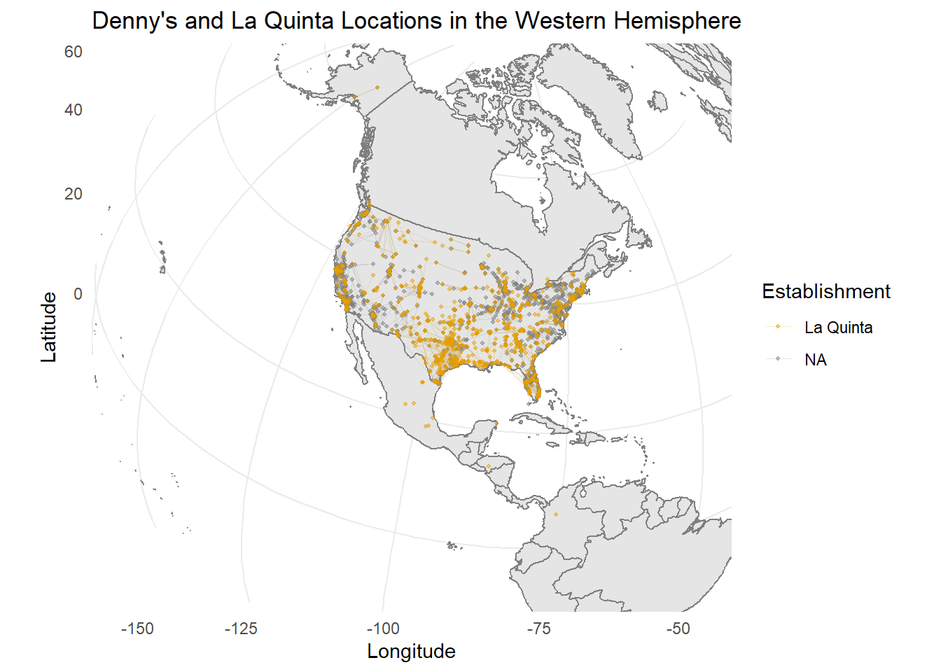
We can plot the locations of the two establishments using a scatter plot, and color the points by the establishment type. Note that the latitude is plotted on the x-axis and the longitude on the y-axis.
The following two questions ask you to create visualizations. These visualizations should follow best practices you learned in class, such as informative titles, axis labels, etc. See http://ggplot2.tidyverse.org/reference/labs.html for help with the syntax. You can also choose different themes to change the overall look of your plots, see http://ggplot2.tidyverse.org/reference/ggtheme.html for help with these.
Filter the data for observations in North Carolina only, and recreate the plot. You should also adjust the transparency of the points, by setting the
alphalevel, so that it’s easier to see the overplotted ones. Visually, does Mitch Hedberg’s joke appear to hold here?Now filter the data for observations in Texas only, and recreate the plot, with an appropriate
alphalevel. Visually, does Mitch Hedberg’s joke appear to hold here?
That’s it for now! In the next lab, we will take a more quantitative approach to answering these questions.
Wrapping up
If you still have some time left, move on to the remaining exercises below. These are optional stretch goals. They are designed to challenge you and hone your skills.
- Recreate the following plot, and interpret what you see in context of the data.
Click to for hints about the library
Hint: You will need to use the
annotation_bordersfunction from the ggplot2 package to add the borders of the world to the plot. You will also need the mapproj package to adjust the projection of the plot.
🧶 ✅ ⬆️ Knit, commit, and push your changes to GitHub with an appropriate commit message. Make sure to commit and push all changed files so that your Git pane is cleared up afterwards and review the md document on GitHub to make sure you’re happy with the final state of your work.