114 LAB: Academic Freedom
Welcome to the Academic Freedom Monitoring Lab! In this lab, we will take on the role of academic freedom analysts, drawing on real-world political indicators from the V-Dem project. Our mission? To evaluate how free scholars are to teach, research, express ideas, and exchange knowledge across time and place.
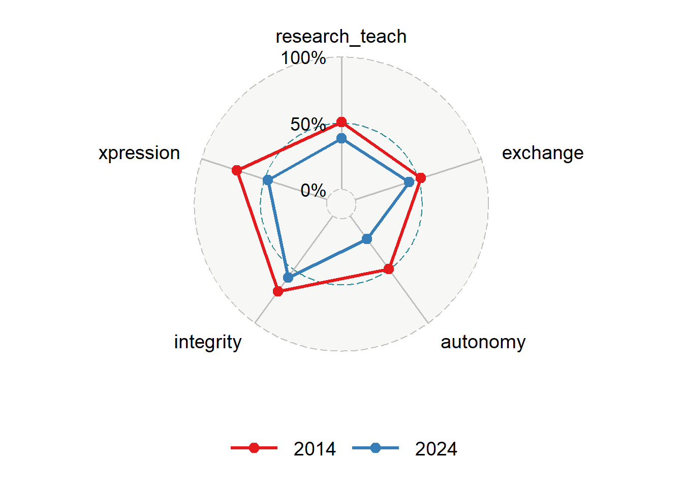
We’ll begin by exploring the 2025 Academic Freedom Index, which highlights concerning trends. In particular, the United States has experienced significant declines across all five dimensions of academic freedom between 2014 and 2024, most sharply in freedom to research and teach and institutional autonomy. According to the index, the U.S. is one of only 34 countries to show a statistically significant decline.
By the end of this lab, you will be able to reconstruct the same kinds of indicator-level visualizations that researchers use to monitor these trends—and place the U.S. within a broader global context.
Getting started and warming up
Packages
We’ll be using vdemdata to access the Academic Freedom Index, as well as the tidyverse and ggradar packages for data manipulation and visualization. Install and load them with:
if (!require("devtools")) install.packages("devtools")
if (!require("vdemdata")) devtools::install_github("vdeminstitute/vdemdata")
if (!require("tidyverse")) install.packages("tidyverse")
if (!require("remotes")) install.packages("remotes")
if (!require("ggradar")) remotes::install_github("ricardo-bion/ggradar")
library(vdemdata)
library(tidyverse)
library(ggradar)
Exercise 1: Academic Freedom in the United States
Let’s begin by examining how academic freedom has changed in the U.S. across five indicators from the latest year available 2025 and the decade before that..
1.1. Filter the vdem dataset to include only the United States in the relevant years. Then select the five indicators that make up the Academic Freedom Index.
vdem <- vdemdata::vdem %>%
  select(country_name, year, v2cafres, v2cafexch, v2cainsaut, v2casurv, v2clacfree)
year_max <- vdemdata::vdem %>%
select(year) %>% max()
year_2010s <- year_max - 10
year_1950s <- year_max - 701.2. Normalize these values so that they fall between 0 and 1, which is the format expected by ggradar().
vdem_scaled <- vdem %>%
  mutate(across(-c(year, country_name), scales::rescale))


u_data_scaled <- vdem %>% # vdem_scaled  %>%
  filter(country_name %in% c("United States of America"), year %in% c(year_1950s, year_2010s, year_max)) %>%
  select(year,
    country_name,
    research_teach = v2cafres,
    exchange = v2cafexch,
    autonomy = v2cainsaut,
    integrity = v2casurv,
    expression = v2clacfree
  ) %>%
  mutate(year = as.factor(year)) %>%
  rename(group = year)
1.3. What do you notice about the raw or rescaled values? Do any indicators show more dramatic declines than others?
Exercise 2: Building the Radar Plot
2.1. Now create a radar plot to compare the United States in 2014 and 2024 across the five indicators.
u_data_scaled %>%
  filter(country_name == "United States of America") %>%
  select(-country_name) %>%
  ggradar(
    grid.min = 0, grid.mid = .5, grid.max = 1,
    group.line.width = 1.2,
    group.point.size = 3,
    legend.position = "bottom"
  ) +
  scale_color_viridis_d()
## Error:
## ! plot.data' contains value(s) < centre.yu_data_scaled %>%
filter(country_name == "United Kingdom") %>%
select(-country_name) %>%
ggradar(
grid.min = 0, grid.mid = .5, grid.max = 1,
group.line.width = 1.2,
group.point.size = 3,
legend.position = "bottom"
) +
scale_color_viridis_d()## Error in `aggregate.data.frame()`:
## ! no rows to aggregate2.2. Interpret the shape of the plot. Which dimensions remained relatively high? Which appear to be collapsing?
Exercise 3: Looking Beyond the U.S.
Let’s now explore whether this decline is unique to the U.S. or part of a broader trend.
3.1. Identify countries where freedom to research and teach declined by more than 0.2 points between 2014 and 2024.
afi_declines <- vdem %>%
  filter(year %in% c(1954, 2014, 2024)) %>%
  select(country_name, year, v2cafres) %>%
  pivot_wider(names_from = year, values_from = v2cafres) %>%
  mutate(diff = `2024` - `2014`) %>%
  filter(diff < -0.2) %>%
  arrange(diff)
3.2. Choose one country from the list and repeat the radar plot analysis for that country.
chosen_country <- "Hungary" # Replace this with your selected country

country_data <- vdem %>%
  filter(country_name == chosen_country, year %in% c(2014, 2024)) %>%
  select(year,
    research_teach = v2cafres,
    exchange = v2cafexch,
    autonomy = v2cainsaut,
    integrity = v2casurv,
    expression = v2clacfree
  ) %>%
  #  mutate(across(-year, scales::rescale)) %>%
  mutate(year = as.factor(year)) %>%
  rename(group = year)

ggradar(country_data,
  grid.min = -3, grid.mid = 0, grid.max = 3,
  group.line.width = 1.2,
  group.point.size = 3,
  legend.position = "bottom"
)
3.3. In what ways does this country’s trajectory resemble or diverge from the U.S. case?