85 ODD: Feature Engineering
85.1 Feature engineering
We prefer simple models when possible, but parsimony does not mean sacrificing accuracy (or predictive performance) in the interest of simplicity
Variables that go into the model and how they are represented are just as critical to success of the model
Feature engineering allows us to get creative with our predictors in an effort to make them more useful for our model (to increase its predictive performance)
85.1.1 Same training and testing sets as before
# Fix random numbers by setting the seed
# Enables analysis to be reproducible when random numbers are used
set.seed(1066)

# Put 80% of the data into the training set
email_split <- initial_split(email, prop = 0.80)

# Create data frames for the two sets:
train_data <- training(email_split)
test_data <- testing(email_split)
85.1.2 A simple approach: mutate()
train_data %>%
  mutate(
    date = date(time),
    dow = wday(time),
    month = month(time)
  ) %>%
  select(time, date, dow, month) %>%
  sample_n(size = 5) # shuffle to show a variety
#> # A tibble: 5 × 4
#>   time                date         dow month
#>   <dttm>              <date>     <dbl> <dbl>
#> 1 2012-02-07 14:17:38 2012-02-07     3     2
#> 2 2012-02-28 19:24:15 2012-02-28     3     2
#> 3 2012-03-12 08:07:31 2012-03-12     2     3
#> 4 2012-01-26 13:58:18 2012-01-26     5     1
#> 5 2012-02-21 08:50:29 2012-02-21     3     2
85.2 Modeling workflow, revisited
Create a recipe for feature engineering steps to be applied to the training data
Fit the model to the training data after these steps have been applied
Using the model estimates from the training data, predict outcomes for the test data
Evaluate the performance of the model on the test data
85.3 Building recipes
85.3.1 Initiate a recipe
email_rec <- recipe(
  spam ~ ., # formula
  data = train_data # data to use for cataloguing names and types of variables
)

summary(email_rec)
#> # A tibble: 21 × 4
#> variable type role source
#> <chr> <list> <chr> <chr>
#> 1 to_multiple <chr [3]> predictor original
#> 2 from <chr [3]> predictor original
#> 3 cc <chr [2]> predictor original
#> 4 sent_email <chr [3]> predictor original
#> 5 time <chr [1]> predictor original
#> 6 image <chr [2]> predictor original
#> 7 attach <chr [2]> predictor original
#> 8 dollar <chr [2]> predictor original
#> 9 winner <chr [3]> predictor original
#> 10 inherit <chr [2]> predictor original
#> 11 viagra <chr [2]> predictor original
#> 12 password <chr [2]> predictor original
#> 13 num_char <chr [2]> predictor original
#> 14 line_breaks <chr [2]> predictor original
#> 15 format <chr [3]> predictor original
#> 16 re_subj <chr [3]> predictor original
#> 17 exclaim_subj <chr [2]> predictor original
#> 18 urgent_subj <chr [3]> predictor original
#> 19 exclaim_mess <chr [2]> predictor original
#> 20 number <chr [3]> predictor original
#> 21 spam <chr [3]> outcome original85.3.2 Remove certain variables
#>
#> ── Recipe ──────────────────────────────────────────────────────────────────────────────────────────
#>
#> ── Inputs
#> Number of variables by role
#> outcome:    1
#> predictor: 20
#>
#> ── Operations
#> • Variables removed: from sent_email
85.3.3 Feature engineer date
#>
#> ── Recipe ──────────────────────────────────────────────────────────────────────────────────────────
#>
#> ── Inputs
#> Number of variables by role
#> outcome:    1
#> predictor: 20
#>
#> ── Operations
#> • Variables removed: from sent_email
#> • Date features from: time
#> • Variables removed: time
85.3.4 Discretize numeric variables
Proceed with major caution! And please be sure to read MacCallum, R. C., Zhang, S., Preacher, K. J., & Rucker, D. D. (2002). On the practice of dichotomization of quantitative variables. Psychological Methods, 7, 19-40. and play around with the demo data from Kris’s website: http://www.quantpsy.org/mzpr.htm
email_rec <- email_rec %>%
  step_cut(cc, attach, dollar, breaks = c(0, 1)) %>%
  step_cut(inherit, password, breaks = c(0, 1, 5, 10, 20))
#>
#> ── Recipe ──────────────────────────────────────────────────────────────────────────────────────────
#>
#> ── Inputs
#> Number of variables by role
#> outcome: 1
#> predictor: 20
#>
#> ── Operations
#> • Variables removed: from sent_email
#> • Date features from: time
#> • Variables removed: time
#> • Cut numeric for: cc, attach, dollar
#> • Cut numeric for: inherit password85.3.5 Create dummy variables
#>
#> ── Recipe ──────────────────────────────────────────────────────────────────────────────────────────
#>
#> ── Inputs
#> Number of variables by role
#> outcome:    1
#> predictor: 20
#>
#> ── Operations
#> • Variables removed: from sent_email
#> • Date features from: time
#> • Variables removed: time
#> • Cut numeric for: cc, attach, dollar
#> • Cut numeric for: inherit password
#> • Dummy variables from: all_nominal() -all_outcomes()85.3.6 Remove zero variance variables
Variables that contain only a single value
#>
#> ── Recipe ──────────────────────────────────────────────────────────────────────────────────────────
#>
#> ── Inputs
#> Number of variables by role
#> outcome:    1
#> predictor: 20
#>
#> ── Operations
#> • Variables removed: from sent_email
#> • Date features from: time
#> • Variables removed: time
#> • Cut numeric for: cc, attach, dollar
#> • Cut numeric for: inherit password
#> • Dummy variables from: all_nominal() -all_outcomes()
#> • Zero variance filter on: all_predictors()85.3.7 All in one place
email_rec <- recipe(spam ~ ., data = email) %>%
  step_rm(from, sent_email) %>%
  step_date(time, features = c("dow", "month")) %>%
  step_rm(time) %>%
  step_cut(cc, attach, dollar, breaks = c(0, 1)) %>%
  step_cut(inherit, password, breaks = c(0, 1, 5, 10, 20)) %>%
  step_dummy(all_nominal(), -all_outcomes()) %>%
  step_zv(all_predictors())
85.4 Building workflows
85.4.2 Define workflow
Workflows bring together models and recipes so that they can be easily applied to both the training and test data.
#> ══ Workflow ════════════════════════════════════════════════════════════════════════════════════════
#> Preprocessor: Recipe
#> Model: logistic_reg()
#>
#> ── Preprocessor ────────────────────────────────────────────────────────────────────────────────────
#> 7 Recipe Steps
#>
#> • step_rm()
#> • step_date()
#> • step_rm()
#> • step_cut()
#> • step_cut()
#> • step_dummy()
#> • step_zv()
#>
#> ── Model ───────────────────────────────────────────────────────────────────────────────────────────
#> Logistic Regression Model Specification (classification)
#>
#> Computational engine: glm
85.4.3 Fit model to training data
email_fit <- email_wflow %>%
  fit(data = train_data)
#> Warning: glm.fit: fitted probabilities numerically 0 or 1 occurredtidy(email_fit) %>% print(n = 31)
#> # A tibble: 31 × 5
#> term estimate std.error statistic p.value
#> <chr> <dbl> <dbl> <dbl> <dbl>
#> 1 (Intercept) -1.11 0.264 -4.19 2.75e- 5
#> 2 image -1.72 0.956 -1.80 7.23e- 2
#> 3 viagra 2.30 182. 0.0126 9.90e- 1
#> 4 num_char 0.0469 0.0271 1.73 8.41e- 2
#> 5 line_breaks -0.00563 0.00151 -3.74 1.87e- 4
#> 6 exclaim_subj -0.0721 0.271 -0.266 7.90e- 1
#> 7 exclaim_mess 0.0101 0.00214 4.72 2.36e- 6
#> 8 to_multiple_X1 -2.83 0.377 -7.49 6.71e-14
#> 9 cc_X.1.68. -0.178 0.468 -0.382 7.03e- 1
#> 10 attach_X.1.21. 2.39 0.381 6.27 3.61e-10
#> 11 dollar_X.1.64. 0.0544 0.222 0.246 8.06e- 1
#> 12 winner_yes 2.20 0.415 5.31 1.11e- 7
#> 13 inherit_X.1.5. -9.14 756. -0.0121 9.90e- 1
#> 14 inherit_X.5.10. 1.95 1.27 1.54 1.23e- 1
#> 15 password_X.1.5. -1.71 0.759 -2.25 2.43e- 2
#> 16 password_X.5.10. -12.4 420. -0.0296 9.76e- 1
#> 17 password_X.10.20. -13.8 812. -0.0170 9.86e- 1
#> 18 password_X.20.28. -13.8 814. -0.0170 9.86e- 1
#> 19 format_X1 -0.802 0.161 -4.99 6.17e- 7
#> 20 re_subj_X1 -2.78 0.400 -6.97 3.25e-12
#> 21 urgent_subj_X1 2.57 1.13 2.27 2.31e- 2
#> 22 number_small -0.659 0.170 -3.87 1.10e- 4
#> 23 number_big 0.199 0.246 0.807 4.20e- 1
#> 24 time_dow_Mon -0.0207 0.300 -0.0690 9.45e- 1
#> 25 time_dow_Tue 0.306 0.273 1.12 2.63e- 1
#> 26 time_dow_Wed -0.204 0.279 -0.731 4.65e- 1
#> 27 time_dow_Thu -0.237 0.297 -0.799 4.24e- 1
#> 28 time_dow_Fri 0.000702 0.284 0.00247 9.98e- 1
#> 29 time_dow_Sat 0.261 0.307 0.851 3.95e- 1
#> 30 time_month_Feb 0.912 0.183 4.97 6.68e- 7
#> 31 time_month_Mar 0.638 0.187 3.41 6.52e- 485.4.4 Make predictions for test data
email_pred <- predict(email_fit, test_data, type = "prob") %>%
  bind_cols(test_data)

email_pred
#> # A tibble: 785 × 23
#>    .pred_0  .pred_1 spam  to_multiple from     cc sent_email time                image attach dollar
#>      <dbl>    <dbl> <fct> <fct>       <fct> <int> <fct>      <dttm>              <dbl>  <dbl>  <dbl>
#>  1   0.948 0.0522   0     0           1         0 0          2012-01-01 04:09:49     0      0      0
#>  2   0.909 0.0914   0     0           1         0 0          2012-01-01 22:00:18     0      0      0
#>  3   0.971 0.0292   0     0           1         0 0          2012-01-02 00:42:16     0      0      5
#>  4   0.887 0.113    0     0           1         0 0          2012-01-01 20:58:14     0      0      0
#>  5   0.992 0.00755  0     0           1         0 0          2012-01-02 02:07:22     0      0     21
#>  6   1.000 0.000432 0     1           1         2 0          2012-01-02 13:09:45     0      0      0
#>  7   0.999 0.000691 0     0           1         1 0          2012-01-02 10:12:51     0      0      0
#>  8   1.000 0.000280 0     1           1         2 0          2012-01-02 16:24:21     0      0      0
#>  9   0.971 0.0292   0     0           1         0 0          2012-01-03 04:34:50     0      0     11
#> 10   0.978 0.0224   0     0           1         0 0          2012-01-03 08:33:28     0      0     18
#> # ℹ 775 more rows
#> # ℹ 12 more variables: winner <fct>, inherit <dbl>, viagra <dbl>, password <dbl>, num_char <dbl>,
#> #   line_breaks <int>, format <fct>, re_subj <fct>, exclaim_subj <dbl>, urgent_subj <fct>,
#> #   exclaim_mess <dbl>, number <fct>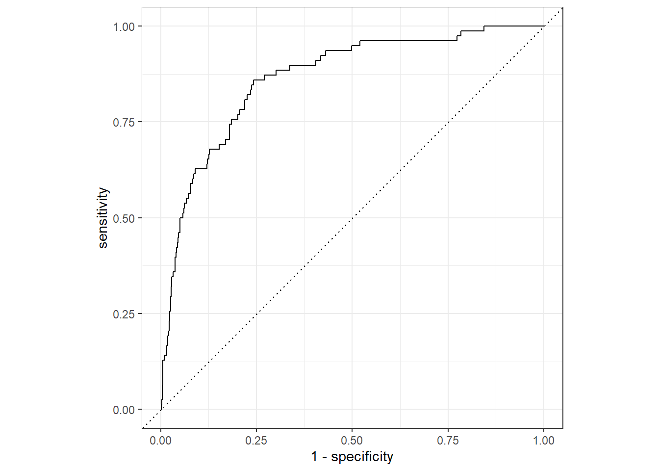
85.5 Making decisions
85.5.1 Cutoff probability: 0.5
Suppose we decide to label an email as spam if the model predicts the probability of spam to be more than 0.5.
cutoff_prob <- 0.5
email_pred %>%
  mutate(
    spam      = if_else(spam == 1, "Email is spam", "Email is not spam"),
    spam_pred = if_else(.pred_1 > cutoff_prob, "Email labelled spam", "Email labelled not spam")
  ) %>%
  count(spam_pred, spam) %>%
  pivot_wider(names_from = spam, values_from = n) %>%
kable(col.names = c("", "Email is not spam", "Email is spam"))| Email is not spam | Email is spam | |
|---|---|---|
| Email labelled not spam | 700 | 68 |
| Email labelled spam | 7 | 10 |
85.5.2 Cutoff probability: 0.25
Suppose we decide to label an email as spam if the model predicts the probability of spam to be more than 0.25.
cutoff_prob <- 0.25
email_pred %>%
  mutate(
    spam      = if_else(spam == 1, "Email is spam", "Email is not spam"),
    spam_pred = if_else(.pred_1 > cutoff_prob, "Email labelled spam", "Email labelled not spam")
  ) %>%
  count(spam_pred, spam) %>%
  pivot_wider(names_from = spam, values_from = n) %>%
kable(col.names = c("", "Email is not spam", "Email is spam"))| Email is not spam | Email is spam | |
|---|---|---|
| Email labelled not spam | 673 | 42 |
| Email labelled spam | 34 | 36 |
85.5.3 Cutoff probability: 0.75
Suppose we decide to label an email as spam if the model predicts the probability of spam to be more than 0.75.
cutoff_prob <- 0.75
email_pred %>%
  mutate(
    spam      = if_else(spam == 1, "Email is spam", "Email is not spam"),
    spam_pred = if_else(.pred_1 > cutoff_prob, "Email labelled spam", "Email labelled not spam")
  ) %>%
  count(spam_pred, spam) %>%
  pivot_wider(names_from = spam, values_from = n) %>%
kable(col.names = c("", "Email is not spam", "Email is spam"))| Email is not spam | Email is spam | |
|---|---|---|
| Email labelled not spam | 703 | 73 |
| Email labelled spam | 4 | 5 |